Page 744 - The Principle of Economics

764
PART TWELVE
SHORT-RUN ECONOMIC FLUCTUATIONS
and, thus, a lower rate of unemployment. In addition, whatever the previous year’s price level happens to be, the higher the price level in the current year, the higher the rate of inflation. Thus, shifts in aggregate demand push inflation and unemployment in opposite directions in the short run—a relationship illustrated by the Phillips curve.
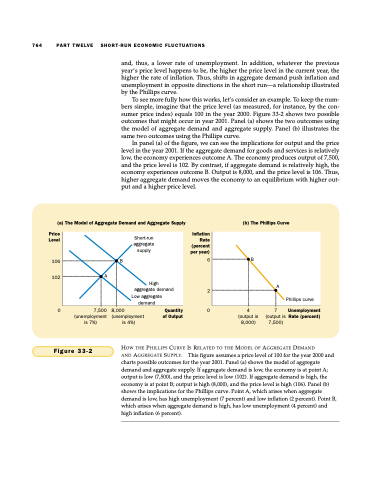
To see more fully how this works, let’s consider an example. To keep the num- bers simple, imagine that the price level (as measured, for instance, by the con- sumer price index) equals 100 in the year 2000. Figure 33-2 shows two possible outcomes that might occur in year 2001. Panel (a) shows the two outcomes using the model of aggregate demand and aggregate supply. Panel (b) illustrates the same two outcomes using the Phillips curve.
In panel (a) of the figure, we can see the implications for output and the price level in the year 2001. If the aggregate demand for goods and services is relatively low, the economy experiences outcome A. The economy produces output of 7,500, and the price level is 102. By contrast, if aggregate demand is relatively high, the economy experiences outcome B. Output is 8,000, and the price level is 106. Thus, higher aggregate demand moves the economy to an equilibrium with higher out- put and a higher price level.
(a) The Model of Aggregate Demand and Aggregate Supply
(b) The Phillips Curve
B
Short-run aggregate supply
A
High aggregate demand
Low aggregate demand
B
A
Phillips curve
Price Level
106 102
0
7,500 8,000
(unemployment (unemployment is 7%) is 4%)
Inflation Rate (percent per year)
6
2
Quantity 0 of Output
4 7
(output is 8,000)
Unemployment (output is Rate (percent)
7,500)
HOW THE PHILLIPS CURVE IS RELATED TO THE MODEL OF AGGREGATE DEMAND
AND AGGREGATE SUPPLY. This figure assumes a price level of 100 for the year 2000 and charts possible outcomes for the year 2001. Panel (a) shows the model of aggregate demand and aggregate supply. If aggregate demand is low, the economy is at point A; output is low (7,500), and the price level is low (102). If aggregate demand is high, the economy is at point B; output is high (8,000), and the price level is high (106). Panel (b) shows the implications for the Phillips curve. Point A, which arises when aggregate demand is low, has high unemployment (7 percent) and low inflation (2 percent). Point B, which arises when aggregate demand is high, has low unemployment (4 percent) and high inflation (6 percent).
Figure 33-2