Page 266 - Introduction to Programming with Java: A Problem Solving Approach

232
Chapter 6
Object-Oriented Programming
45
40
35
30
25
20
15
10
5 0
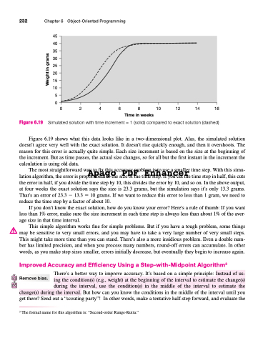
Figure 6.19
Simulated solution with time increment = 1 (solid) compared to exact solution (dashed)
0 2 4 6 8 10 12 14 16
Time in weeks
Figure 6.19 shows what this data looks like in a two-dimensional plot. Alas, the simulated solution doesn’t agree very well with the exact solution. It doesn’t rise quickly enough, and then it overshoots. The reason for this error is actually quite simple. Each size increment is based on the size at the beginning of the increment. But as time passes, the actual size changes, so for all but the first instant in the increment the calculation is using old data.
The most straightforward way to fix this accuracy problem is to use a smaller time step. With this simu-
Apago PDF Enhancer
lation algorithm, the error is proportional to the size of the time step. If you cut the time step in half, this cuts the error in half, if you divide the time step by 10, this divides the error by 10, and so on. In the above output, at four weeks the exact solution says the size is 23.3 grams, but the simulation says it’s only 13.3 grams. That’s an error of 23.3 􏰂 13.3 􏰁 10 grams. If we want to reduce this error to less than 1 gram, we need to reduce the time step by a factor of about 10.
If you don’t know the exact solution, how do you know your error? Here’s a rule of thumb: If you want less than 1% error, make sure the size increment in each time step is always less than about 1% of the aver- age size in that time interval.
This simple algorithm works fine for simple problems. But if you have a tough problem, some things may be sensitive to very small errors, and you may have to take a very large number of very small steps. This might take more time than you can stand. There’s also a more insidious problem. Even a double num- ber has limited precision, and when you process many numbers, round-off errors can accumulate. In other words, as you make step sizes smaller, errors initially decrease, but eventually they begin to increase again.
Improved Accuracy and Efficiency Using a Step-with-Midpoint Algorithm3
Remove bias.
There’s a better way to improve accuracy. It’s based on a simple principle: Instead of us- ing the condition(s) (e.g., weight) at the beginning of the interval to estimate the change(s) during the interval, use the condition(s) in the middle of the interval to estimate the
change(s) during the interval. But how can you know the conditions in the middle of the interval until you get there? Send out a “scouting party”! In other words, make a tentative half-step forward, and evaluate the
3 The formal name for this algorithm is: “Second-order Runge-Kutta.”
Weight in grams