Page 703 - The Principle of Economics

To sum up, this story about shifts in aggregate demand has two important lessons:
N In the short run, shifts in aggregate demand cause fluctuations in the economy’s output of goods and services.
N In the long run, shifts in aggregate demand affect the overall price level but do not affect output.
CASE STUDY TWO BIG SHIFTS IN AGGREGATE DEMAND: THE GREAT DEPRESSION AND WORLD WAR II
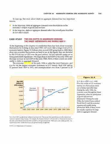
At the beginning of this chapter we established three key facts about economic fluctuations by looking at data since 1965. Let’s now take a longer look at U.S. economic history. Figure 31-9 shows data on real GDP going back to 1900. Most short-run economic fluctuations are hard to see in this figure; they are dwarfed by the 25-fold rise in GDP over the past century. Yet two episodes jump out as being particularly significant—the large drop in real GDP in the early 1930s and the large increase in real GDP in the early 1940s. Both of these events are attrib- utable to shifts in aggregate demand.
The economic calamity of the early 1930s is called the Great Depression, and it is by far the largest economic downturn in U.S. history. Real GDP fell by 27 percent from 1929 to 1933, and unemployment rose from 3 percent to 25
CHAPTER 31 AGGREGATE DEMAND AND AGGREGATE SUPPLY 723
The Great Depression
The World War II Boom
Real GDP
Real GDP (billions of 1992 dollars)
8,000 4,000 2,000 1,000
500
250
1900 1910 1920 1930 1940 1950 1960 1970 1980 1990 2000
Figure 31-9
U.S. REAL GDP SINCE 1900. Over the course of U.S. economic history, two fluctuations stand out as being especially large. During the early 1930s, the economy went through the Great Depression, when the production of goods and services plummeted. During the early 1940s, the United States entered World War II, and the economy experienced rapidly rising production. Both of these events are usually explained by large shifts in aggregate demand.
NOTE: Real GDP is graphed here using a proportional scale. This means that equal distances on the vertical axis represent equal percentage changes. For example, the distance between 1,000 and 2,000 (a 100 percent increase) is the same as the distance between 2,000 and 4,000 (a 100 percent increase). With such a scale, stable growth—say, 3 percent per year—would show up as an upward-sloping straight line.
SOURCE: U.S. Department of Commerce.