Page 52 - Kennemerland VOC ship, 1664 - Published Reports

NAUTICAL ARCHAEOLOGY, 4.2
182
1 TI 111 1Va IVb IVc V VI VIII IX XI 11
I1 0.400 111 0.328
IVa 0.356
IVb 0.236
1vc 0.373
V 0.188
VI 0.190
VlIl 0.098 IX 0.119 XI 0.109
1
0.373 1
0,520 0.514 1
0.271 0.481 0.419 1
0.540 0.500 0.968 0.419 1
0.115 0.039 0.096 0.070 0.096 1
0.204 0.267 0.200 0.192 0.194 0.106 1 0.036 0.024 0.023 0.029 0.023 0.316 0.081 0.089 0.022 0,111 0.061 0,111 0.308 0.103 0.120 0.167 0.182 0.211 0.176 0.079 0.120
1
0.265 1
0.032 0,069 1
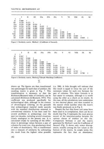
Figure 5. Similarity matrix
Method 1 (Coefficient of Jaccard).
1 I1 111 IVa IVb IVc V VI VIlI 1x XI 11
I1 0.567 1
111 om0.6441
1Va 0 3 7 8 1Vb 0.533 IVC 0.589
V 0-422 VI 0.478 VllI 0.389 IX 0.422 XI 0.456
0.733 0.800 1
0.611 0.844 0,800 1
0.744 0.789 0.989 0.800 1
0.400 0.456 0.478 0.556 0.478 1
0.567 0.756 0.689 0.767 0.678 0.533 1 0.411 0.544 0.522 0622 0.522 0.711 0622 0.433 0.511 0.556 0.656 0.556 0.700 0.611 0,511 0-722 0.700 0-833 0.689 0.611 0,756
1
0.722 1
0.667 0.700 1
Figure 6. Similarity matrix, Methodp/(Simple Matching Coefficient).
7T
drawn up. The figures are then transformed into percentages for each class of artefact; the resulting matrix is given in Fig. 7. This transformation is necessary so that the RobinsonlBrainerd index of similarity can be calculated (Robinson & Brainerd, 1951). This coefficient was produced specifically for archaeological data, although in the context of chronological ordering, on the grounds that archaeological material rarely accords with the standard distributions assumed in conventional statistics. It has been used for several problems in archaeology over the past two decades, including several situations closely analogous to the present one. It is calculated simply by summing all the differ- ences in percentage values between a pair of columns for every row, thus producing a kind of index of dissimilarity. This is transformed into a measure of similarity by subtracting the result from the highest value possible
-
(i.e. 200). A little thought will indicate that this result is equal to twice the sum of the minimum values for each row between the pair of columns. This latter formula is in fact easier to compute, although it is worth using the other as a check on its results. In this case, all the calculations were undertaken to two decimal places, and then rounded to the nearest whole number when the matrix was finally produced, as in Fig. 8.
Despite the fact that fewer unit areas have been used in its compilation, there can be no doubt that Fig. 8 represents the most precise record of the interrelationship between the various classes of artefact on this site. Comparison between it and the matrix generated by Method 1 and the Coefficient of Jaccard (Fig. 5) shows only minor discrep- ancies, notably among the low values at the bottom of the matrix. In simple terms this represents the fact that an abundance/