Page 310 - The ROV Manual - A User Guide for Remotely Operated Vehicles 2nd edition

302 CHAPTER 12 Sensor Theory
1
mrs 0.5
mh
hc
h
–1 –0.5
–0.5
–1
0.5 1
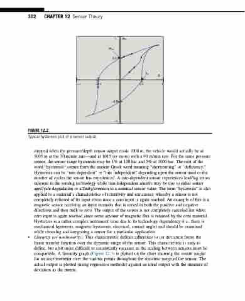
FIGURE 12.2
Typical hysteresis plot of a sensor output.
stopped when the pressure/depth sensor output reads 1000 m, the vehicle would actually be at 1005 m at the 30 m/min rate—and at 1015 (or more) with a 90 m/min rate. For the same pressure sensor, the sensor range hysteresis may be 1% at 100 bar and 5% at 1000 bar. The root of the word “hysteresis” comes from the ancient Greek word meaning “shortcoming” or “deficiency.” Hysteresis can be “rate dependent” or “rate independent” depending upon the sensor used or the number of cycles the sensor has experienced. A rate-dependent sensor experiences lead/lag errors inherent in the sensing technology while rate-independent sensors may be due to either sensor age/cycle degradation or affinity/aversion to a nominal sensor value. The term “hysteresis” is also applied to a material’s characteristics of retentivity and remanence whereby a sensor is not completely relieved of its input stress once a zero input is again reached. An example of this is a magnetic sensor receiving an input intensity that is varied in both the positive and negative directions and then back to zero. The output of the sensor is not completely canceled out when zero input is again reached since some amount of magnetic flux is retained by the core material. Hysteresis is a rather complex instrument issue due to its technology dependency (i.e., there is mechanical hysteresis, magnetic hysteresis, electrical, contact angle) and should be examined while choosing and integrating a sensor for a particular application.
• Linearity (or nonlinearity): This characteristic defines adherence to (or deviation from) the linear transfer function over the dynamic range of the sensor. This characteristic is easy to define, but a bit more difficult to consistently measure as the scaling between sensors must be comparable. A linearity graph (Figure 12.3) is plotted on the chart showing the sensor output for an accelerometer over the various points throughout the dynamic range of the sensor. The actual output is plotted (using regression methods) against an ideal output with the measure of deviation as the metric.