Page 46 - CITN 2017 Journal

3.2 Model specification
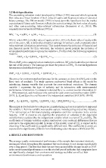
The accounting valuation model developed by Ohlson (1995) was used which represents
firm value as a linear function of book value of equity and the present value of expected
future earnings. The Ohlson model (1995) is based upon the hypothesis that the market
expectations of future cash flows are reflected in current earnings, the book value of equity,
and other non-accounting value-relevant information (Semenova et al., 2010). The
originally derived model of Olshon (1995) is

MV = α + α BV + α AE + α v ..............................................................................(1)
1
it
2
0
3 it
it
it
Where: where MV is market value of equity at time t, BV is the book value of equity at the
t t
end of the year t, AE is defined as abnormal earnings for period t, and v represents other
t t
value-relevant information (error term). This model stresses the inclusion of financial and
non-financial model for firm valuation; the valuation model permits the inclusion of
environmental performance a proxy for variable v. For this study the following regression
t
model is
SMP = β + β BVS + β EPS + ε ................................................................(2)
i,t 0 1 i, t 2 i, t i, t
Where SMP is the company's share market price at time t. BV is the book value per share at
i,t
i,t
the end of the period t. The earnings per share for period t is EPS . To test the hypotheses
i,t
the regression model is developed;
SMP = β + β BVS + β EPS + β ENVS + ε ..........................................................(3)
i,t 0 1 i, t 2 i, t 3 i,t i,…
The proxy for environmental performance for the company at time t is ENVS and ε is the
i,t
Error term of residuals. The study captures unobserved fixed effects in the model by
introducing dummy variable that accounts for cross-sectional variations. The dummy
variable 1 represents the type of industry and its interaction with environmental
performance information. A company is denoted by i, i.e. a cross-section observation (i=
1...100companies), and t indicates time periods for each cross-section observation (2009 -
2013). β , β and β are the coefficients of the independent variables (BVS, EPS, ENVS).
1
3
2
SMP = β + β BVS + β EPS + β ENVS + β I + β5(I ENVS )+ε ..............................(4)
i,t 0 1 i, t 2 i, t 3 i,t 4 i,t i,t i,t i,t
The sample is divided into two categories; manufacturing and service industry to represent
the variable I. Dummy variable was used to capture manufacturing and service industry.
“I” is represented as 1 for manufacturing companies and 0 for companies in the service
2
industry. If R is closer to one signifies the proportion of variation in the dependent
variable that is explained by the independent variable which is a test of H1 and H2 . The
0 0
coefficients of dummy variables explain unobserved cross sectional differences that are
relevant to the explanatory model. In terms of this model, a test of H2 is carried out by
0
observing if the coefficient β is significantly different zero. The coefficients β and β are
1
3
2
expected to be significantly different from 0 indicating value relevance of BVS and EPS.
4. RESULT AND DISCUSSION

The average yearly environmental performance of the sample has remained relatively
unchanged which strengthens the argument that such ratings do not change significantly
over a long period. The fact that there has not been an incredible change except in 2010
in the environmental performance over the studied period indicates that companies have
not significantly changed their environmental strategy such that can affect their
environmental performance and reputation.
39