Page 4 - jamshid

True value and an estimate All estimates and max Bias as function of state Average error
2 2 max a Q t (s, a) − max a Q ∗ (s, a)
Q ∗ (s, a) max a Q t (s, a) 1 +0.61
0 0 0 −0.02
Q t (s, a) Double-Q estimate
−1
−2 −2
2 Q ∗ (s, a) 2 max a Q t (s, a) 1 max a Q t (s, a) − max a Q ∗ (s, a) +0.47
Q t (s, a) 0 +0.02
Double-Q estimate
0 0 −1

4 4 4 max a Q t (s, a)−
Q t (s, a) max a Q t (s, a) max a Q ∗ (s, a)
2 2 2 +3.35
0 0 0 −0.02
Q ∗ (s, a) Double-Q estimate
−6 −4 −2 0 2 4 6 −6 −4 −2 0 2 4 6 −6 −4 −2 0 2 4 6
state state state
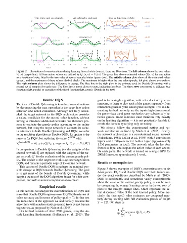
Figure 2: Illustration of overestimations during learning. In each state (x-axis), there are 10 actions. The left column shows the true values
V ∗(s) (purple line). All true action values are defined by Q ∗(s, a) = V ∗(s). The green line shows estimated values Q(s, a) for one action
as a function of state, fitted to the true value at several sampled states (green dots). The middle column plots show all the estimated values
(green), and the maximum of these values (dashed black). The maximum is higher than the true value (purple, left plot) almost everywhere.
The right column plots shows the difference in orange. The blue line in the right plots is the estimate used by Double Q-learning with a
second set of samples for each state. The blue line is much closer to zero, indicating less bias. The three rows correspond to different true
functions (left, purple) or capacities of the fitted function (left, green). (Details in the text)

Double DQN goal is for a single algorithm, with a fixed set of hyperpa-
The idea of Double Q-learning is to reduce overestimations rameters, to learn to play each of the games separately from
by decomposing the max operation in the target into action interaction given only the screen pixels as input. This is a de-
selection and action evaluation. Although not fully decou- manding testbed: not only are the inputs high-dimensional,
pled, the target network in the DQN architecture provides the game visuals and game mechanics vary substantially be-
a natural candidate for the second value function, without tween games. Good solutions must therefore rely heavily
having to introduce additional networks. We therefore pro- on the learning algorithm — it is not practically feasible to
pose to evaluate the greedy policy according to the online overfit the domain by relying only on tuning.
network, but using the target network to estimate its value. We closely follow the experimental setting and net-
In reference to both Double Q-learning and DQN, we refer work architecture outlined by Mnih et al. (2015). Briefly,
to the resulting algorithm as Double DQN. Its update is the the network architecture is a convolutional neural network
same as for DQN, but replacing the target Y t DQN with (Fukushima, 1988; LeCun et al., 1998) with 3 convolution
Y t DoubleDQN ≡ R t+1 +γQ(S t+1 , argmax Q(S t+1 , a; θ t ), θ ) . layers and a fully-connected hidden layer (approximately
−
1.5M parameters in total). The network takes the last four
t
a
frames as input and outputs the action value of each action.
In comparison to Double Q-learning (4), the weights of the
second network θ are replaced with the weights of the tar- On each game, the network is trained on a single GPU for
0
t
200M frames, or approximately 1 week.
get network θ for the evaluation of the current greedy pol-
−
t
icy. The update to the target network stays unchanged from
DQN, and remains a periodic copy of the online network. Results on overoptimism
This version of Double DQN is perhaps the minimal pos-
sible change to DQN towards Double Q-learning. The goal Figure 3 shows examples of DQN’s overestimations in six
is to get most of the benefit of Double Q-learning, while Atari games. DQN and Double DQN were both trained un-
keeping the rest of the DQN algorithm intact for a fair com- der the exact conditions described by Mnih et al. (2015).
parison, and with minimal computational overhead. DQN is consistently and sometimes vastly overoptimistic
about the value of the current greedy policy, as can be seen
Empirical results by comparing the orange learning curves in the top row of
plots to the straight orange lines, which represent the ac-
In this section, we analyze the overestimations of DQN and tual discounted value of the best learned policy. More pre-
show that Double DQN improves over DQN both in terms of cisely, the (averaged) value estimates are computed regu-
value accuracy and in terms of policy quality. To further test larly during training with full evaluation phases of length
the robustness of the approach we additionally evaluate the T = 125, 000 steps as
algorithms with random starts generated from expert human
trajectories, as proposed by Nair et al. (2015). T
Our testbed consists of Atari 2600 games, using the Ar- 1 X argmax Q(S t , a; θ) .
cade Learning Environment (Bellemare et al., 2013). The T a
t=1