Page 467 - Physics Coursebook 2015 (A level)

Chapter 29: Alternating currents
QUESTIONS
5 If the Y-sensitivity and time-base for the trace shown in Figure 29.7 are 5 V/cm and 10 ms/cm, what are the amplitude, period and frequency of the signal to the Y-input?
6 Draw the c.r.o. trace for a sinusoidal voltage of frequency 100 Hz and amplitude 10 V, when the time-base is 10 ms/cm and the Y-sensitivity is 10 V/cm.
Power and a.c.
We use mains electricity to supply us with energy. If the current and voltage are varying all the time, does this mean that the power is varying all the time too? The answer to this is yes. You may have noticed that some fluorescent lamps flicker continuously, especially if you observe them out of the corner of your eye. A tungsten filament lamp would flicker too, but the frequency of the mains has been chosen so that the filament does not have time to cool down noticeably between peaks in the supply.
BOX 29.2: Comparing a.c. and d.c
Because power supplied by an alternating current
is varying all the time, we need to have some way of describing the average power which is being supplied. To do this, we compare an alternating current with a direct current, and try to find the direct current that supplies the same average power as the alternating current.
Figure 29.8 shows how this can be done in practice. Two lamps are placed side by side; one is connected
Figure 29.8 Comparing direct and alternating currents that supply the same power. The lamps are equally bright.
Root-mean-square values
There is a mathematical relationship between the peak value V0 of the alternating voltage and a d.c. voltage which delivers the same average electrical power. The d.c. voltage is about 70% of V0. (You might have expected it to be about half, but it is more than this, because of the shape of the sine graph.) This steady d.c. voltage is known as the root- mean-square (r.m.s.) value of the alternating voltage. In the same way, we can think of the root-mean-square value of an alternating current, Irms:
(The lamps in Box 29.2 are the ‘resistive loads’.) A full analysis, which we will come to shortly, shows that Irms is related to I0 by:
The root-mean-square value of an alternating current is that steady current which delivers the same average power as the a.c. to a resistive load.
I = I / 2 or I ≈ 0.707 × I rms 0 rms
0
This is where the factor of 70% comes from. Note that this
factor only applies to sinusoidal alternating currents.
to an a.c. supply (on the right) and the other to a d.c. supply (the batteries on the left). The a.c. supply is adjusted so that the two lamps are equally bright, indicating that the two supplies are providing energy at the same average rate. The output voltages are then compared on the double-beam oscilloscope.
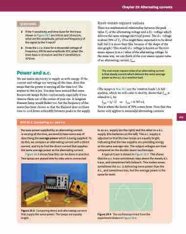
A typical trace is shown in Figure 29.9. This shows that the a.c. trace sometimes rises above the steady d.c. trace, and sometimes falls below it. This makes sense: sometimes the a.c. is delivering more power than the d.c., and sometimes less, but the average power is the same for both.
Figure 29.9 The oscilloscope trace from the experiment shown in Figure 29.8.
455