Page 546 - Physics Coursebook 2015 (A level)

534
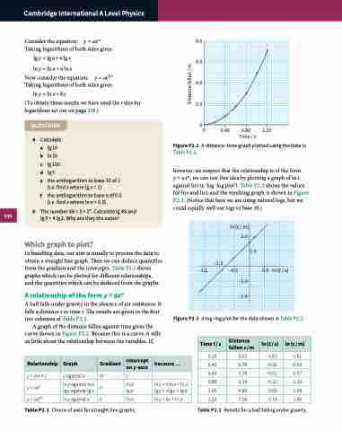
Figure P2.2 A distance–time graph plotted using the data in Table P2.2.
however, we suspect that the relationship is of the form
y = axn, we can test this idea by plotting a graph of ln s against ln t (a ‘log–log plot’). Table P2.2 shows the values for ln s and ln t, and the resulting graph is shown in Figure P2.3. (Notice that here we are using natural logs, but we could equally well use logs to base 10.)
ln (s / m) 2.0
1.0
Cambridge International A Level Physics
Consider the equation: y = axn Taking logarithms of both sides gives:
lgy = lga+nlgx lny = lna+nlnx
8.0 6.0 4.0 2.0
+ +
+
Distance fallen / m
y = aekx
(To obtain these results we have used the rules for
Now consider the equation:
Taking logarithms of both sides gives:
lny = lna+kx
logarithms set out on page 318.)
+
QUESTIONS
4 Calculate:
a lg10
b ln10
c lg100
d lg5
e the antilogarithm to base 10 of 1 (i.e.findxwherelgx=1)
f the antilogarithm to base e of 0.5 (i.e. find x where ln x = 0.5)
5 The number 48 = 3 × 24. Calculate lg 48 and lg3 + 4 lg2. Why are they the same?
+ 0+
0 0.40
0.80 1.20 Time / s
Which graph to plot?
In handling data, our aim is usually to process the data to obtain a straight line graph. Then we can deduce quantities from the gradient and the intercepts. Table P2.1 shows graphs which can be plotted for different relationships, and the quantities which can be deduced from the graphs.
A relationship of the form y = axn
A ball falls under gravity in the absence of air resistance. It
falls a distance s in time t. The results are given in the first two columns of Table P2.2.
A graph of the distance fallen against time gives the curve shown in Figure P2.2. Because this is a curve, it tells us little about the relationship between the variables. If,
–1.0
Relationship
Graph
Gradient
Intercept on y-axis
because ...
ln y = n ln x + ln a lgy = nlgx + lga
ln y = kx + ln a
Time t / s 0.20
0.40 0.60 0.80 1.00 1.20
Table P2.2
Distance fallens/m
0.20 0.78 1.76 3.14 4.90 7.05
ln (t / s) −1.61
−0.92 −0.51 −0.22
0.00 0.18
ln (s / m) −1.61
−0.25 0.57 1.14 1.59 1.95
y=mx+c yagainstx m c
ln a lga
y = aekx ln y against x k
Table P2.1 Choice of axes for straight-line graphs.
y = axn ln y against ln x n lgy against lgx
ln a
Figure P2.3
A log–log plot for the data shown in Table P2.2.
–1.5
–0.5
0.5 ln (t / s)
–1.0 –2.0
Results for a ball falling under gravity.