Page 547 - Physics Coursebook 2015 (A level)

From this graph the gradient is equal to the value of n, the power of t:
n = gradient = (2.55 − (−1.4)) (0.5 − (−1.5))
= 3.95 2.0
= 1.98 ≈ 2.0
So the equation is of the form s = at2. The intercept on the
y-axis is equal to ln a, so: ln a = 1.6
By taking the antilogarithm we get: a = 4.95ms−2 ≈ 5.0ms−2
If we think of the equation for free fall s = 12 gt2, the constant a = 12 g. But g = 9.8 m s−2, which is consistent with the value we get for our constant.
A relationship of the form y = aekx
A current flows from a charged capacitor when it is
connected in a circuit with a resistor. The current decreases exponentially with time (the same pattern we see in radioactive decay).
Figure P2.4 shows the circuit and Table P2.3 shows typical values of current I and time t from such an experiment.
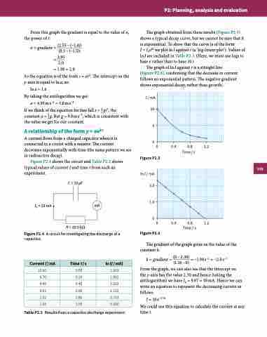
The graph obtained from these results (Figure P2.5) shows a typical decay curve, but we cannot be sure that it is exponential. To show that the curve is of the form
I = I0ekt we plot ln I against t (a ‘log-linear plot’). Values of ln I are included in Table P2.3. (Here, we must use logs to base e rather than to base 10.)
The graph of ln I against t is a straight line
(Figure P2.6), confirming that the decrease in current follows an exponential pattern. The negative gradient shows exponential decay, rather than growth.
I0 = 10 mA
mA
capacitor.
Current I/mA 10.00
6.70 4.49 3.01 2.02 1.35
Time t/s 0.00 0.20 0.40 0.60 0.80 1.00
ln(I/mA) 2.303 1.902 1.502 1.102 0.703 0.300
The gradient of the graph gives us the value of the constant k:
k = gradient = (0 − 2.30) = −1.98 s−1 ≈ −2.0 s−1 (1.16 − 0)
From the graph, we can also see that the intercept on the y-axis has the value 2.30 and hence (taking the antilogarithm) we have I0 = 9.97 ≈ 10 mA. Hence we can write an equation to represent the decreasing current as follows:
I = 10e−2.0t
We could use this equation to calculate the current at any time t.
C = 10 μF
R = 20.0 kΩ
Figure P2.4 A circuit for investigating the discharge of a
0
0.4 0.8 1.2 Time / s
Table P2.3 Results from a capacitor discharge experiment.
I / mA 10
5
0
Figure P2.5
ln I / mA 2.0
1.0 0
0.4 0.8 1.2 Time / s
Figure P2.6
0
P2: Planning, analysis and evaluation
535