Page 470 - The Principle of Economics

480 PART SEVEN
ADVANCED TOPIC
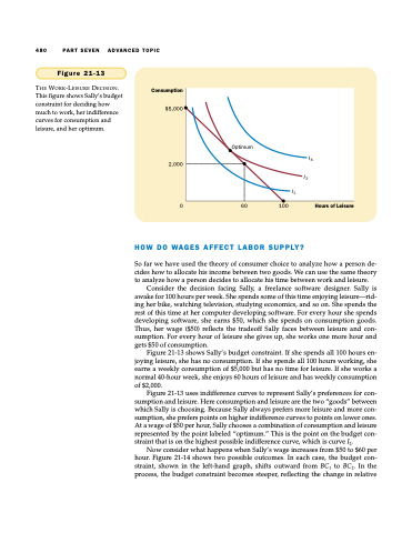
Figure 21-13
THE WORK-LEISURE DECISION. This figure shows Sally’s budget constraint for deciding how much to work, her indifference curves for consumption and leisure, and her optimum.
Consumption
$5,000
2,000
0 60 100
Optimum
I3
I2 I1
Hours of Leisure
HOW DO WAGES AFFECT LABOR SUPPLY?
So far we have used the theory of consumer choice to analyze how a person de- cides how to allocate his income between two goods. We can use the same theory to analyze how a person decides to allocate his time between work and leisure.
Consider the decision facing Sally, a freelance software designer. Sally is awake for 100 hours per week. She spends some of this time enjoying leisure—rid- ing her bike, watching television, studying economics, and so on. She spends the rest of this time at her computer developing software. For every hour she spends developing software, she earns $50, which she spends on consumption goods. Thus, her wage ($50) reflects the tradeoff Sally faces between leisure and con- sumption. For every hour of leisure she gives up, she works one more hour and gets $50 of consumption.
Figure 21-13 shows Sally’s budget constraint. If she spends all 100 hours en- joying leisure, she has no consumption. If she spends all 100 hours working, she earns a weekly consumption of $5,000 but has no time for leisure. If she works a normal 40-hour week, she enjoys 60 hours of leisure and has weekly consumption of $2,000.
Figure 21-13 uses indifference curves to represent Sally’s preferences for con- sumption and leisure. Here consumption and leisure are the two “goods” between which Sally is choosing. Because Sally always prefers more leisure and more con- sumption, she prefers points on higher indifference curves to points on lower ones. At a wage of $50 per hour, Sally chooses a combination of consumption and leisure represented by the point labeled “optimum.” This is the point on the budget con- straint that is on the highest possible indifference curve, which is curve I2.
Now consider what happens when Sally’s wage increases from $50 to $60 per hour. Figure 21-14 shows two possible outcomes. In each case, the budget con- straint, shown in the left-hand graph, shifts outward from BC1 to BC2. In the process, the budget constraint becomes steeper, reflecting the change in relative