Page 19 - Algebra

2.5. Graphing Linear Equations
For graphing functions, you need to understand the rate of change and slope. In a graph, when x is the
independent variable, and y is the dependent variable, the rate of change is given by:
Rate of change =
𝐶h𝑎𝑛𝑔𝑒 𝑖𝑛 𝑦
𝐶h𝑎𝑛𝑔𝑒 𝑖𝑛 𝑥
In graphs, the rate of change is the slope of the line (m) passing through points, (x1, y1) and (x2, y2)
Slope of the line passing through
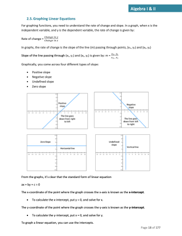
Graphically, you come across four different types of slope:
• • • •
From the graphs, it’s clear that the standard form of linear equation
ax + by + c = 0
The x-coordinate of the point where the graph crosses the x-axis is known as the x-intercept.
• To calculate the x-intercept, put y = 0, and solve for x.
The y-coordinate of the point where the graph crosses the y-axis is known as the y-intercept.
• To calculate the y-intercept, put x = 0, and solve for y. To graph a linear equation, you can use the intercepts.
Negative slope
(x1, y1) and (x2, y2) is given by: m = 𝑦2− 𝑦1 𝑥2− 𝑥1
Positive slope
Undefined slope
Zero slope
Page 18 of 177
Algebra I & II