Page 77 - Algorithms Notes for Professionals

Chapter 15: Applications of Dynamic

Programming

The basic idea behind dynamic programming is breaking a complex problem down to several small and simple
problems that are repeated. If you can identify a simple subproblem that is repeatedly calculated, odds are there is
a dynamic programming approach to the problem.

As this topic is titled Applications of Dynamic Programming, it will focus more on applications rather than the process
of creating dynamic programming algorithms.

Section 15.1: Fibonacci Numbers

Fibonacci Numbers are a prime subject for dynamic programming as the traditional recursive approach makes a lot
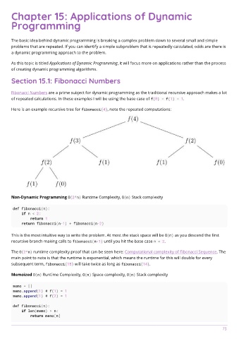
of repeated calculations. In these examples I will be using the base case of f(0) = f(1) = 1.

Here is an example recursive tree for fibonacci(4), note the repeated computations:

Non-Dynamic Programming O(2^n) Runtime Complexity, O(n) Stack complexity

def fibonacci(n):
if n < 2:
return 1
return fibonacci(n-1) + fibonacci(n-2)

This is the most intuitive way to write the problem. At most the stack space will be O(n) as you descend the first
recursive branch making calls to fibonacci(n-1) until you hit the base case n < 2.

The O(2^n) runtime complexity proof that can be seen here: Computational complexity of Fibonacci Sequence. The
main point to note is that the runtime is exponential, which means the runtime for this will double for every
subsequent term, fibonacci(15) will take twice as long as fibonacci(14).

Memoized O(n) Runtime Complexity, O(n) Space complexity, O(n) Stack complexity

memo = []
memo.append(1) # f(1) = 1
memo.append(1) # f(2) = 1

def fibonacci(n):
if len(memo) > n:
return memo[n]

colegiohispanomexicano.net – Algorithms Notes 73