Page 3 - SUBHARADEV SEN AND AHMED

IAPQR Transactions

systems. Finally, Section 6 concludes with some future research areas
in this direction.

2. THE BIVARIATE FINITE RANGE DISTRIBUTION

In this section, we introduce and study some basic properties of a
bivariate extension of finite range distribution, mentioned in the
introduction. Let X and Y be two random variables having low to
moderate dependency. Before proceeding further, let us recall the
basic definition of the Farlie-Gumbel-Morgenstern (FGM) method for
constructing bivariate distribution.

If X has marginal pdf, f X(x), and cdf, F X(x), and Y has marginal pdf,
f Y(y), and cdf, F Y(y), then the joint distribution function of (X, Y) is
given by

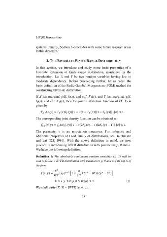
, , 1 1 1 , | | 1.

The corresponding joint density function can be obtained as
, , 1 2 1 2 1 , | | 1.

The parameter α is an association parameter. For reference and
additional properties of FGM family of distributions, see Hutchinson
and Lai ([2], 1990). With the above definition in mind, we now
proceed in introducing BVFR distribution with parameters p, θ and α.
We have the following definition.

Definition 1: The absolutely continuous random variables (X, Y) will be
said to follow a BVFR distribution with parameters p, θ and α if its pdf is of
the form

, 1 2 2 ,

0 , ; , 0; | | 1. (3)
We shall write (X, Y) ~ BVFR (p, θ, α).

75