Page 224 - thinkpython

202 Appendix B. Analysis of Algorithms

run slower in this case. A common way to avoid this problem is to analyze the worst
case scenario. It is sometimes useful to analyze average case performance, but that’s
usually harder, and it might not be obvious what set of cases to average over.

• Relative performance also depends on the size of the problem. A sorting algorithm
that is fast for small lists might be slow for long lists. The usual solution to this
problem is to express run time (or number of operations) as a function of problem
size, and group functions into categories depending on how quickly they grow as
problem size increases.

The good thing about this kind of comparison is that it lends itself to simple classification
of algorithms. For example, if I know that the run time of Algorithm A tends to be pro-
2
portional to the size of the input, n, and Algorithm B tends to be proportional to n , then I
expect A to be faster than B, at least for large values of n.
This kind of analysis comes with some caveats, but we’ll get to that later.

B.1 Order of growth

Suppose you have analyzed two algorithms and expressed their run times in terms of the
size of the input: Algorithm A takes 100n + 1 steps to solve a problem with size n; Algo-
2
rithm B takes n + n + 1 steps.
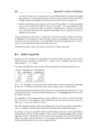
The following table shows the run time of these algorithms for different problem sizes:
Input Run time of Run time of
size Algorithm A Algorithm B
10 1 001 111
100 10 001 10 101
1 000 100 001 1 001 001
10 000 1 000 001 100 010 001

At n = 10, Algorithm A looks pretty bad; it takes almost 10 times longer than Algorithm
B. But for n = 100 they are about the same, and for larger values A is much better.
2
The fundamental reason is that for large values of n, any function that contains an n term
will grow faster than a function whose leading term is n. The leading term is the term with
the highest exponent.
For Algorithm A, the leading term has a large coefficient, 100, which is why B does better
than A for small n. But regardless of the coefficients, there will always be some value of n
2
where an > bn, for any values of a and b.
The same argument applies to the non-leading terms. Even if the run time of Algorithm A
were n + 1000000, it would still be better than Algorithm B for sufficiently large n.
In general, we expect an algorithm with a smaller leading term to be a better algorithm for
large problems, but for smaller problems, there may be a crossover point where another
algorithm is better. The location of the crossover point depends on the details of the algo-
rithms, the inputs, and the hardware, so it is usually ignored for purposes of algorithmic
analysis. But that doesn’t mean you can forget about it.