Page 227 - Ms Excel Note and Workbook

MICROSOFT EXCEL NOTE AND WORKBOOK

PRACTICE QUESTION 5

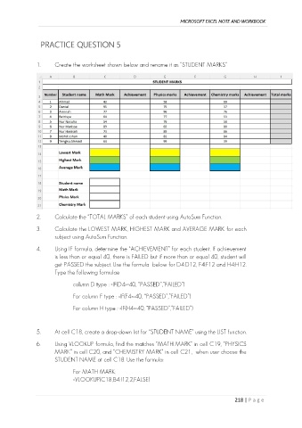
1. Create the worksheet shown below and rename it as “STUDENT MARKS”

2. Calculate the “TOTAL MARKS” of each student using AutoSum Function.

3. Calculate the LOWEST MARK, HIGHEST MARK and AVERAGE MARK for each
subject using AutoSum Function.

4. Using IF formula, determine the “ACHIEVEMENT” for each student. If achievement
is less than or equal 40, there is FAILED but if more than or equal 40, student will
get PASSED the subject. Use the formula below for D4:D12, F4:F12 and H4:H12.
Type the following formulae

column D type : =IF(D4>=40, “PASSED”,”FAILED”)

For column F type : =IF(F4>=40, “PASSED”,”FAILED”)

For column H type : =IF(H4>=40, “PASSED”,”FAILED”)

5. At cell C18, create a drop-down list for “STUDENT NAME” using the LIST function.

6. Using VLOOKUP formula, find the matches “MATH MARK” in cell C19, “PHYSICS
MARK” in cell C20, and “CHEMISTRY MARK” in cell C21, when user choose the
STUDENT NAME at cell C18. Use the formula:
For MATH MARK:
=VLOOKUP(C18,B4:I12,2,FALSE)

218 | P a g e