Page 166 - Linear Models for the Prediction of Animal Breeding Values

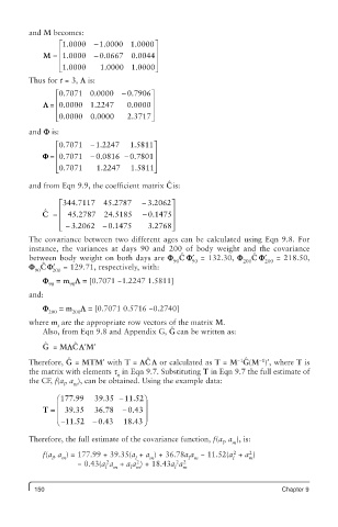
and M becomes:
é é 1 0000 -1 0000 1 0000 ù
.
.
.
ê ú
.
.
M = 1 0000 - 0 0667 0 0044 ú
.
ê
ê ë 1 0000 1 0000 1 0000ú û
.
.
.
Thus for t = 3, L is:
é 0 7071 0 0000 - 0 7906ù
.
.
.
ê ú
.
L = 0 0000 1 2247 0 0000 ú
.
.
ê
ê ë 0 0000 0 0000 2 3717ú û
.
.
.
7
and F is:
é 0 7071 - 1 2247 1 5811ù
.
.
.
ê
F = 0 7071 - 0 0816 - 0 7801 ú ú
.
.
.
ê
ê ë 0 7071 1 2247 1 58811ú û
.
.
.
ˆ
and from Eqn 9.9, the coefficient matrix C is:
é 344 7117 45 2787 - 3 2062. ù
.
.
ˆ
C = ê ê 45 2787 24 5185 - 0 1475 ú ú
.
.
.
ê ë - 3 2062 - 0 14775 3 2768ú û
.
.
.
The covariance between two different ages can be calculated using Eqn 9.8. For
instance, the variances at days 90 and 200 of body weight and the covariance
between body weight on both days are F C F′ = 132.30, F 200 C F′ = 218.50,
ˆ
ˆ
90
90
200
ˆ
F C F′ = 129.71, respectively, with:
90 200
F =m L = [0.7071 −1.2247 1.5811]
90 90
and:
F =m L = [0.7071 0.5716 −0.2740]
200 200
where m are the appropriate row vectors of the matrix M.
i
ˆ
Also, from Eqn 9.8 and Appendix G, G can be written as:
ˆ
G = MLCL′M′
ˆ
−1 ˆ
ˆ
ˆ
−1
Therefore, G = MTM′ with T = LC L or calculated as T = M G(M )′, where T is
the matrix with elements t in Eqn 9.7. Substituting T in Eqn 9.7 the full estimate of
ij
the CF, f(a , a ), can be obtained. Using the example data:
l m
æ177 99. 39 35 -11 52 ö
.
.
T = ç ç 39 35 36 78 - 0 43 ÷ ÷ ÷
.
.
.
ç ÷
.
.
.
è -11 52 - 0 43 18 43 ø
Therefore, the full estimate of the covariance function, f(a , a ), is:
l m
2
2
f(a , a ) = 177.99 + 39.35(a + a ) + 36.78a a − 11.52(a + a )
l m l m l m l m
− 0.43(a a + a a ) + 18.43a a
2
2 2
2
l m l m l m
150 Chapter 9