Page 238 - Linear Models for the Prediction of Animal Breeding Values

2
2
with G = Is s or Is u if a sire or an animal model is being fitted in a univariate situation.
They presented equations for the calculation of the matrices in Eqn 13.4, which are outlined
below. The calculation of most of these matrices involves P (see Eqn 13.2) and it is initially
jk
described. P , the response in the kth category under the conditions of the jth row, is:
jk
P = F(t − a ) − F(t − a ); k = 1, m − 1; j = 1,..., s (13.5)
jk k j k−1 j
where a = (x b + z u), with x and z being the jth row of X and Z, respectively.
j j j j j
This equation is no different from that in Section 13.2.1, but it shows that the dis-
tribution of response probabilities by category is a function of the distance between
a and the threshold. Similarly, the height of the normal curve at t (Eqn 13.1) under
j k
the conditions of the jth row becomes:
f = f(t − a ) (13.6)
jk k j
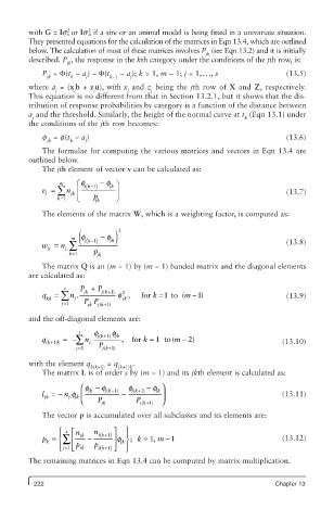
The formulae for computing the various matrices and vectors in Eqn 13.4 are
outlined below.
The jth element of vector v can be calculated as:

j å
v = m n ç æ f j( k- ) 1 - f jk ö ÷ (13.7)
jk
k=1 ç è p jk ÷ ø
The elements of the matrix W, which is a weighting factor, is computed as:
jk) 2
m f
w = n j ∑ jk ( ( − ) 1 − f (13.8)
jj .
k=1 p jk
The matrix Q is an (m − 1) by (m − 1) banded matrix and the diagonal elements
are calculated as:
s
jk
(
2
=
1
q kk å n . P + P j k+ )1 f , for k =1 to ( m - ) (13.9)
j
jk
j=1 PP j k+ )1
(
jk
and the off-diagonal elements are:
s
−
q k ( +1 k ) =− ∑ n j. f jk ( +1 ) f jk , for k = 1 to ( m 2 ) (13.10)
=
j 1 P jk+1 )
(
with the element q = q .
k(k+1) (k+1)k
The matrix L is of order s by (m − 1) and its jkth element is calculated as:
⎞
(
(
l =− j jk ⎜ ⎛ f jk − f j k− ) 1 − f jk+ ) 1 − f jk ⎟ (13.11)
.
jk n f
⎝ P jk P jk+ ) 1 ⎠
(
The vector p is accumulated over all subclasses and its elements are:
⎧ s ⎡ n n ⎤ ⎫
⎪
⎪
(
p = ⎨∑ ⎢ jk − j k+ ) 1 (13.12)
k p p ⎥ ⎥f jk ⎬ ; k = 1, m − 1
j ⎣ ⎢
(
⎭
⎩ ⎪ =1 jk j k+ ) 1 ⎦ ⎪
The remaining matrices in Eqn 13.4 can be computed by matrix multiplication.
222 Chapter 13