Page 273 - Linear Models for the Prediction of Animal Breeding Values

−1
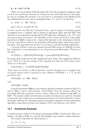
q = q + Einf (¶L/¶q) (15.4)
n
There are two problems with this approach. First, the parameters might go nega-
tive and one would want estimates of variances to stay essentially positive. One popu-
lar way of avoiding this property is to note that at a maximum of the likelihood the
first differentials are zero and to manipulate Eqns 15.1 and 15.2 in the form:
2
(n − p)s = (y − Xb − Za) ′ (y) (15.5)
e
2 −1 22 −1 2
a e
qs = a ′ A a + trace[C A ]s (15.6)
2 2
e a
so that it can be seen that s is estimated from a sum of squares of residuals and s
is estimated from a weighted sum of squares of predicted values and their PEV. This
algorithm is an expectation maximization (EM) algorithm (Dempster et al., 1977) and
successive iterates are positive. The algorithm can be written in the form of the updat-
ing formula if Einf is replaced by a matrix that depends on the information derived,
as if one could directly observe the residuals and breeding values rather than predict-
ing them. This algorithm can be slow to converge in animal breeding applications.
A second problem is that the expected second differentials are difficult to calcu-
late. Sometimes it is recommended to use observed second differentials. These are of
the form:
1
2
(¶L /¶q ¶q ) = −y ′ P(¶V/¶q )P(¶V/¶q )Py + ( 2 )trace[P(¶V/¶q )P(¶V/¶q )]
i j i j i j
but again, these terms involve the complicated trace terms. One suggestion (Gilmour
et al., 1995) is to use the average of the expected and observed information terms.
These are of the form:
2
1
A(¶L /¶q ¶q ) = −( ){y ′ P(¶V/¶q )P(¶V/¶q )Py}
i j 2 i j
These terms are similar to y ¢ Py in that they could be thought of as a weighted sum
of squares matrix with y replaced by two columns (¶V/¶q )Py (i = 1, 2). In this
i
particular case:
2 2
e e
(¶V/¶s )Py = (y − Xb − Za)/s
and:
2 2
a a
(¶V/¶s )Py = Za/s
As in the formation of Einf, we can construct and base an iterative scheme on Eqn 15.3
2
and on Ainf, a matrix with elements −A(¶L /¶q ¶q ). Once the iterative scheme has
i j
−1
converged, then the asymptotic variance matrix of q can be estimated from Ainf or
−1
Einf . The animal model and estimation procedure introduced can easily be extended
to deal with other models, just as prediction procedures can be developed for a variety
of models. Software for estimating variance parameters using this average information
algorithm is described by Jensen and Madsen (1997) and Gilmour et al. (2003).
15.7 Numerical Example

Consider the data in Table 15.2 for the pre-weaning gain (WWG) of beef calves. This is very
similar to the data of Table 3.1, with the data changed to give positive variance estimates.
The model to describe the observations is:
y = p + a + e
ijk i j ijk
Estimation of Genetic Parameters 257