Page 300 - Linear Models for the Prediction of Animal Breeding Values

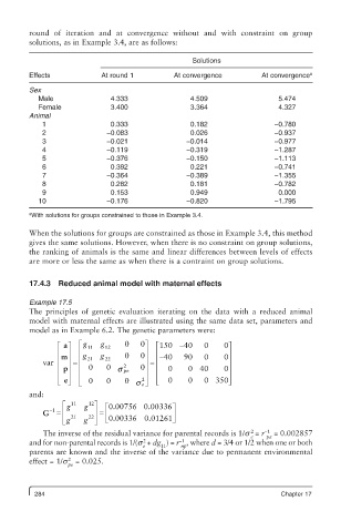
round of iteration and at convergence without and with constraint on group
solutions, as in Example 3.4, are as follows:
Solutions

Effects At round 1 At convergence At convergence a
Sex
Male 4.333 4.509 5.474
Female 3.400 3.364 4.327
Animal
1 0.333 0.182 −0.780
2 −0.083 0.026 −0.937
3 −0.021 −0.014 −0.977
4 −0.119 −0.319 −1.287
5 −0.376 −0.150 −1.113
6 0.392 0.221 −0.741
7 −0.364 −0.389 −1.355
8 0.282 0.181 −0.782
9 0.153 0.949 0.000
10 −0.176 −0.820 −1.795
a With solutions for groups constrained to those in Example 3.4.

When the solutions for groups are constrained as those in Example 3.4, this method
gives the same solutions. However, when there is no constraint on group solutions,
the ranking of animals is the same and linear differences between levels of effects
are more or less the same as when there is a contraint on group solutions.

17.4.3 Reduced animal model with maternal effects

Example 17.5
The principles of genetic evaluation iterating on the data with a reduced animal
model with maternal effects are illustrated using the same data set, parameters and
model as in Example 6.2. The genetic parameters were:
é aù ég 11 g 12 0 0ù é150 -40 0 ù 0
ê ú ê g g 0 0 ú ê -40 90 0 0 ú
m
var ê ú = ê 21 22 ú = ê ú
ê pú ê 0 0 2 p e 0ú ê 0 0 40 ú 0
ê ú ê ê s ú ê ú
ë û ê ë 0 0 0 s ú ë 0 0 0 350 û
e
2
eû
and:
é g 11 g 12 ù é0.00756 0.00336ù
G = ê 21 22 ú = ê ú
-1
ë êg g ú û ë ë 0.00336 0.01261 û
2
−1
The inverse of the residual variance for parental records is 1/s = r = 0.002857
e pa
2
−1
and for non-parental records is 1/(s + dg ) = r , where d = 3/4 or 1/2 when one or both
e 11 np
parents are known and the inverse of the variance due to permanent environmental
2
effect = 1/s = 0.025.
pe
284 Chapter 17