Page 309 - Linear Models for the Prediction of Animal Breeding Values

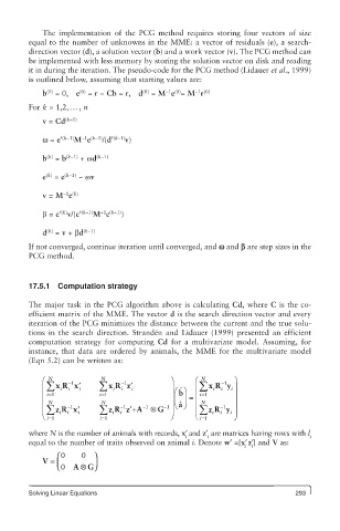
The implementation of the PCG method requires storing four vectors of size
equal to the number of unknowns in the MME: a vector of residuals (e), a search-
direction vector (d), a solution vector (b) and a work vector (v). The PCG method can
be implemented with less memory by storing the solution vector on disk and reading
it in during the iteration. The pseudo-code for the PCG method (Lidauer et al., 1999)
is outlined below, assuming that starting values are:
(0)
(0)
(0)
−1 (0)
−1 (0)
b = 0, e = r − Cb = r, d = M e = M r
For k = 1,2,..., n
v = Cd (k−1)
ω = e′ (k−1) M e /(d′ (k−1) v)
−1 (k−1)
(k)
b = b (k−1) + wd (k−1)
e = e (k−1) − wv
(k)
v = M e
−1 (k)
b = e′ v/(e′ (k−1) M e )
−1 (k−1)
(k)
d = v + βd (k−1)
(k)
If not converged, continue iteration until converged, and w and b are step sizes in the
PCG method.

17.5.1 Computation strategy

The major task in the PCG algorithm above is calculating Cd, where C is the co -
efficient matrix of the MME. The vector d is the search direction vector and every
iteration of the PCG minimizes the distance between the current and the true solu-
tions in the search direction. Strandén and Lidauer (1999) presented an efficient
computation strategy for computing Cd for a multivariate model. Assuming, for
instance, that data are ordered by animals, the MME for the multivariate model
(Eqn 5.2) can be written as:

æ N N ö æ N - ö
-1
1
ç å xR x′ i å x R -1 z′ i ÷ æ ö ˆ ç å xR y i ÷
i
i
i
i
i
i
ç i 1 i 1 ÷ ç ÷ = ç i= 1 ÷
b
=
=
÷ç ÷
ç N N -1 è ø ç N ÷
ˆ a
-
ç ç å zR x′ i å z R z A -1 Ä G ÷ ÷ ç ç å å zR y ÷
+ ′
-1
1
-1
i ÷
i
i
i
i
i
i
è i i=1 i 1 ø i è =1 ø
=
where N is the number of animals with records, x′ and z′ are matrices having rows with l
i i i
equal to the number of traits observed on animal i. Denote w′ =[x′z′] and V as:
i i
⎛ 0 0 ⎞
V = ⎜ ⎝ 0 A ⊗ G⎠ ⎟
Solving Linear Equations 293