Page 341 - Linear Models for the Prediction of Animal Breeding Values

Appendix G: Calculating F, a Matrix of

Legendre Polynomials Evaluated at

Different Ages or Time Periods

The matrix F is of order t (the number of days in milk or ages) by k (where k is the
order of fit) with element f = f (a ) equals the jth Legendre polynomial evaluated at
ij j t
the tth standardized age or days in milk (DIM). Thus a is the tth DIM or age stand-
t
ardized to the interval for which the polynomials are defined. Kirkpatrick et al. (1990,
1994) used Legendre polynomials that span the interval −1 to +1. Defining d and
min
d as the first and latest DIM on the trajectory, DIM d can be standardized to a as:
max t t
a = −1 + 2(d − d )/(d − d )
t t min max min
In matrix notation, F = ML, where M is the matrix containing the polynomials of the
standardized DIM values and L is a matrix of order k containing the coefficients of
Legendre polynomials. The elements of M can be calculated as m = (a (j−1) , i = 1,...t;
ij i
j = 1,...k). For instance, given that k = 5 and that t = 3 (three standardized DIM), M is:
1 ⎡ a a 2 a 3 a ⎤
4
⎢ 1 1 1 1 ⎥
M = 1 ⎢ a 2 a 2 2 a 3 2 a 4 2 ⎥
⎢ 2 3 4 ⎥
⎣ ⎢ 1 a 3 a 3 a 3 a 3 ⎦ ⎥
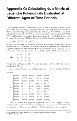
Using the fat yield data in Table 9.1 as an illustration, with ten DIM, the vector of
standardized DIM is:

a′ = [−1.0 −0.7778 −0.5556 −0.3333 −0.1111 0.1111 0.3333 0.5556 0.7778 1.0]
and M is:
⎡ 1.0000 −1.0000 1.0000 −1.0000 1.0000⎤
⎢ ⎥
⎢ 1.0000 −0.7778 0.6049 −0.44705 0.3660 ⎥
⎢ 1.0000 − 0.5556 0.3086 − 0.1715 0.0953⎥
⎢ ⎥
⎢ 1.0000 − 0.3333 0.11111 − 0.0370 0.0123 ⎥
⎢ 1.0000 − 0.1111 0.0123 − 0.0014 0.0002 ⎥
M = ⎢ ⎥
⎢ 1.0000 0.11111 0.0123 0.0014 0.0002 ⎥
⎢ 1.0000 0.3333 0.1111 0.0370 0.0123 ⎥
⎢ ⎥
⎢ 1.0000 0.5556 0.3086 0.1715 0.0953⎥
0
⎢ ⎥ ⎥
⎢ 1.0000 0.7778 0.6049 0.4705 0.3660 ⎥
⎢ ⎣ 1.00000 1.0000 1.0000 1.0000 1.0000⎥ ⎦
Next, the matrix L of Legendre polynomials needs to be computed. The jth
Legendre polynomial evaluated at age t(P (t)) can in general be evaluated by the
j
formula given by Abramowitz and Stegun (1965). In general, for the j integral:

© R.A. Mrode 2014. Linear Models for the Prediction of Animal Breeding Values, 325
3rd Edition (R.A. Mrode)