Page 153 - Understanding Machine Learning

12.4 Summary 135

hinge

0 − 1
1

y〈w, x〉
1

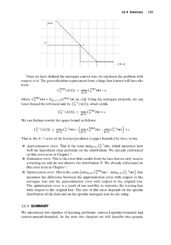
Once we have defined the surrogate convex loss, we can learn the problem with
respect to it. The generalization requirement from a hinge loss learner will have the
form
hinge hinge
L (A(S)) ≤ min L (w) +
,
D D
w∈H
hinge hinge
where L (w) = E (x,y)∼D [ (w,(x, y))]. Using the surrogate property, we can
D
lower bound the left-hand side by L 0−1 (A(S)), which yields
D
L 0−1 (A(S)) ≤ min L hinge (w) +
.
D D
w∈H
We can further rewrite the upper bound as follows:

0−1 0−1 hinge 0−1
L (A(S)) ≤ min L (w) + min L (w) − min L (w) +
.
D D D D
w∈H w∈H w∈H
That is, the 0−1 error of the learned predictor is upper bounded by three terms:
Approximation error: This is the term min w∈H L 0−1 (w), which measures how
D
well the hypothesis class performs on the distribution. We already elaborated
on this error term in Chapter 5.
Estimation error: This is the error that results from the fact that we only receive
a training set and do not observe the distribution D. We already elaborated on
this error term in Chapter 5.

hinge 0−1
Optimization error: This is the term min w∈H L (w) − min w∈H L (w) that
D D
measures the difference between the approximation error with respect to the
surrogate loss and the approximation error with respect to the original loss.
The optimization error is a result of our inability to minimize the training loss
with respect to the original loss. The size of this error depends on the specific
distribution of the data and on the specific surrogate loss we are using.

12.4 SUMMARY

We introduced two families of learning problems: convex-Lipschitz-bounded and
convex-smooth-bounded. In the next two chapters we will describe two generic