Page 162 - Understanding Machine Learning

Regularization and Stability
144

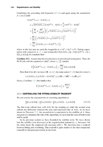
Combining the preceding with Equation (13.14) and again using the assumption
β ≤ λm/2 yield

(i)
(A(S ),z i ) − (A(S),z i )
β
(i) (i) 2
≤ 2βØ (A(S),z i ) A(S ) − A(S) + A(S ) − A(S)
2
2 2
4β 8β
(i)

≤ + (A(S),z i ) + (A(S ),z )
λm (λm) 2
2
8β
(i)

≤ (A(S),z i ) + (A(S ),z )
λm
24β (i)

≤ (A(S),z i ) + (A(S ),z ) ,
λm
2
2
2
where in the last step we used the inequality (a + b) ≤ 3(a + b ). Taking expec-
(i)
tation with respect to S, z , i and noting that E[ (A(S),z i )] = E[ (A(S ), z )] =
E[L S (A(S))], we conclude that:
Corollary 13.7. Assume that the loss function is β-smooth and nonnegative. Then, the
2 2β
RLM rule with the regularizer λ w ,where λ ≥ , satisfies
m

48β
(i)
E (A(S ),z i ) − (A(S),z i ) ≤ E[L S (A(S))].
λm
Note that if for all z we have (0, z) ≤ C, for some scalar C > 0, then for every S,
2
2
L S (A(S)) ≤ L S (A(S)) + λ A(S) ≤ L S (0) + λ 0 = L S (0) ≤ C.
Hence, Corollary 13.7 also implies that

48β C
(i)
E (A(S ),z i ) − (A(S),z i ) ≤ .
λm
13.4 CONTROLLING THE FITTING-STABILITY TRADEOFF
We can rewrite the expected risk of a learning algorithm as

E[L D (A(S))] = E[L S (A(S))] + E[L D (A(S)) − L S (A(S))]. (13.15)
S S S
The first term reflects how well A(S) fits the training set while the second term
reflects the difference between the true and empirical risks of A(S). As we have
shown in Theorem 13.2, the second term is equivalent to the stability of A.Since
our goal is to minimize the risk of the algorithm, we need that the sum of both terms
will be small.
In the previous section we have bounded the stability term. We have shown
that the stability term decreases as the regularization parameter, λ, increases. On
the other hand, the empirical risk increases with λ. We therefore face a tradeoff
between fitting and overfitting. This tradeoff is quite similar to the bias-complexity
tradeoff we discussed previously in the book.