Page 193 - Understanding Machine Learning

15.4 Duality 175

The reason SVM relies on the hinge loss and not on the ramp loss is that the
hinge loss is convex and, therefore, from the computational point of view, min-
imizing the hinge loss can be performed efficiently. In contrast, the problem of
minimizing the ramp loss is computationally intractable.

15.3 OPTIMALITY CONDITIONS AND “SUPPORT VECTORS”*

The name “Support Vector Machine” stems from the fact that the solution of hard-
SVM, w 0 , is supported by (i.e., is in the linear span of) the examples that are exactly
at distance 1/ w 0 from the separating hyperplane. These vectors are therefore
called support vectors.Tosee this,we rely on Fritz John optimality conditions.
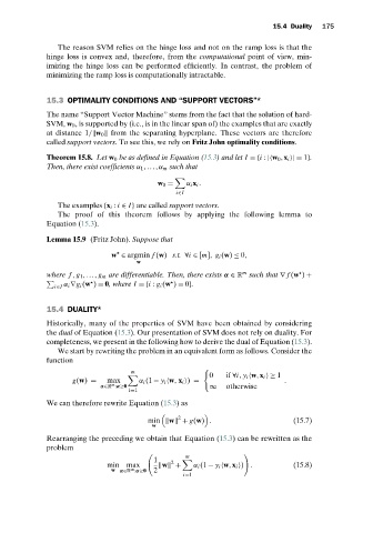
Theorem 15.8. Let w 0 be as defined in Equation (15.3)and let I ={i : | w 0 ,x i | = 1}.
Then, there exist coefficients α 1 ,...,α m such that

w 0 = α i x i .
i∈I
The examples {x i : i ∈ I} are called support vectors.
The proof of this theorem follows by applying the following lemma to
Equation (15.3).

Lemma 15.9 (Fritz John). Suppose that

w ∈ argmin f (w) s.t. ∀i ∈ [m], g i (w) ≤ 0,
w
m
where f ,g 1 ,...,g m are differentiable. Then, there exists α ∈ R such that ∇ f (w ) +

α i ∇g i (w ) = 0,where I ={i : g i (w ) = 0}.
i∈I
15.4 DUALITY*
Historically, many of the properties of SVM have been obtained by considering
the dual of Equation (15.3). Our presentation of SVM does not rely on duality. For
completeness, we present in the following how to derive the dual of Equation (15.3).
We start by rewriting the problem in an equivalent form as follows. Consider the
function
m
0 if ∀i, y i w,x i ≥ 1
g(w) = max α i (1 − y i w, x i ) = .
m
α∈R :α≥0 ∞ otherwise
i=1
We can therefore rewrite Equation (15.3)as

2
min w + g(w) . (15.7)
w
Rearranging the preceding we obtain that Equation (15.3) can be rewritten as the
problem
m
1 2
min max w + α i (1 − y i w,x i ) . (15.8)
m
w α∈R :α≥0 2
i=1