Page 205 - Understanding Machine Learning

16.4 Summary 187

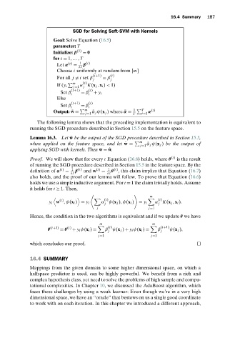
SGD for Solving Soft-SVM with Kernels
Goal: Solve Equation (16.5)
parameter: T
Initialize: β (1) = 0
for t = 1,...,T
Let α (t) = 1 β (t)
λt
Choose i uniformly at random from [m]
(t+1) (t)
For all j = i set β = β
j j
m
(t)
If (y i j=1 α K(x j ,x i ) < 1)
j
(t+1) (t)
Set β = β + y i
i i
Else
(t+1) (t)
Set β = β
i i
m 1 T (t)

Output: ¯ w = ¯ α j ψ(x j )where ¯α = α
j=1 T t=1
The following lemma shows that the preceding implementation is equivalent to
running the SGD procedure described in Section 15.5 on the feature space.
Lemma 16.3. Let ˆ w be the output of the SGD procedure described in Section 15.5,
m

when applied on the feature space, and let ¯ w = j=1 ¯ α j ψ(x j ) be the output of
applying SGD with kernels. Then ¯ w = ˆ w.
Proof. We will show that for every t Equation (16.6) holds, where θ (t) is the result
of running the SGD procedure described in Section 15.5 in the feature space. By the
(t)
definition of α (t) = 1 β (t) and w (t) = 1 θ , this claim implies that Equation (16.7)
λt λt
also holds, and the proof of our lemma will follow. To prove that Equation (16.6)
holds we use a simple inductive argument. For t = 1 the claim trivially holds. Assume
it holds for t ≥ 1. Then,
m
! "
7 8
(t) (t) (t)
y i w ,ψ(x i ) = y i α ψ(x j ),ψ(x i ) = y i α K(x j ,x i ).
j
j
j j=1
Hence, the condition in the two algorithms is equivalent and if we update θ we have
m m
(t) (t+1)
(t+1)
(t)
θ = θ + y i ψ(x i ) = β ψ(x j ) + y i ψ(x i ) = β ψ(x j ),
j j
j=1 j=1
which concludes our proof.
16.4 SUMMARY
Mappings from the given domain to some higher dimensional space, on which a
halfspace predictor is used, can be highly powerful. We benefit from a rich and
complex hypothesis class, yet need to solve the problems of high sample and compu-
tational complexities. In Chapter 10, we discussed the AdaBoost algorithm, which
faces these challenges by using a weak learner: Even though we’re in a very high
dimensional space, we have an “oracle” that bestows on us a single good coordinate
to work with on each iteration. In this chapter we introduced a different approach,