Page 248 - Understanding Machine Learning

Neural Networks
230

That is, the input to v t+1, j is a weighted sum of the outputs of the neurons in V t that
are connected to v t+1, j , where weighting is according to w, and the output of v t+1, j
is simply the application of the activation function σ on its input.
Layers V 1 ,...,V T −1 are often called hidden layers. The top layer, V T , is called
the output layer. In simple prediction problems the output layer contains a single
neuron whose output is the output of the network.
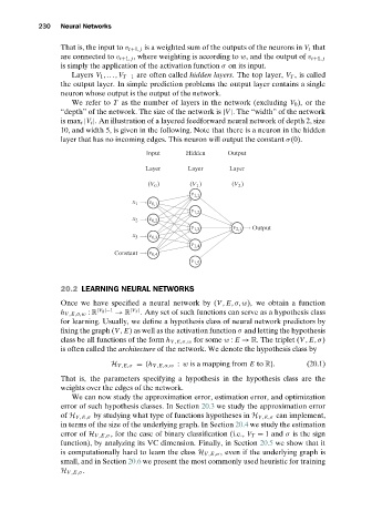
We refer to T as the number of layers in the network (excluding V 0 ), or the
“depth” of the network. The size of the network is |V|. The “width” of the network
is max t |V t |. An illustration of a layered feedforward neural network of depth 2, size
10, and width 5, is given in the following. Note that there is a neuron in the hidden
layer that has no incoming edges. This neuron will output the constant σ(0).

Input Hidden Output
Layer Layer Layer

(V ) (V ) (V )
0
1
2
v 1,1
x 1 v 0,1
v 1,2
x 2 v 0,2
v 1,3 v 2,1 Output
x 3 v 0,3
v 1,4
Constant v 0,4
v 1,5

20.2 LEARNING NEURAL NETWORKS

Once we have specified a neural network by (V , E,σ,w), we obtain a function
h V ,E,σ,w : R |V 0 |−1 → R |V T | . Any set of such functions can serve as a hypothesis class
for learning. Usually, we define a hypothesis class of neural network predictors by
fixing the graph (V , E) as well as the activation function σ and letting the hypothesis
class be all functions of the form h V ,E,σ,w for some w : E → R. The triplet (V , E,σ)
is often called the architecture of the network. We denote the hypothesis class by

H V,E,σ ={h V,E,σ,w : w is a mapping from E to R}. (20.1)

That is, the parameters specifying a hypothesis in the hypothesis class are the
weights over the edges of the network.
We can now study the approximation error, estimation error, and optimization
error of such hypothesis classes. In Section 20.3 we study the approximation error
of H V ,E,σ by studying what type of functions hypotheses in H V ,E,σ can implement,
in terms of the size of the underlying graph. In Section 20.4 we study the estimation
error of H V,E,σ , for the case of binary classification (i.e., V T = 1and σ is the sign
function), by analyzing its VC dimension. Finally, in Section 20.5 we show that it
is computationally hard to learn the class H V,E,σ , even if the underlying graph is
small, and in Section 20.6 we present the most commonly used heuristic for training
H V ,E,σ .