Page 278 - Understanding Machine Learning

Online Learning
260

therefore obtain the update rule

(t)
w (t) if y t w ,x t > 0
(t+1)
w =
w (t) + ηy t x t otherwise
(t)
Denote by M the set of rounds in which sign( w ,x t ) = y t . Note that on round t,
the prediction of the Perceptron can be rewritten as

(t)
p t = sign( w ,x t ) = sign η y i x i ,x t .
i∈M:i<t
This form implies that the predictions of the Perceptron algorithm and the set M
do not depend on the actual value of η as long as η> 0. We have therefore obtained
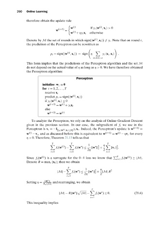
the Perceptron algorithm:

Perceptron
initialize: w 1 = 0
for t = 1,2,...,T
receive x t
(t)
predict p t = sign( w ,x t )
(t)
if y t w ,x t ≤ 0
w (t+1) = w (t) + y t x t
else
w (t+1) = w (t)

To analyze the Perceptron, we rely on the analysis of Online Gradient Descent
given in the previous section. In our case, the subgradient of f t we use in the
Perceptron is v t =−1 [y t w ,x t ≤0] t x t . Indeed, the Perceptron’s update is w (t+1) =
y
(t)
w (t) − v t , and as discussed before this is equivalent to w (t+1) = w (t) − ηv t for every
η> 0. Therefore, Theorem 21.15 tells us that
T T T
1 η
(t) 2 2
f t (w ) − f t (w ) ≤ w + v t .
2
2
2η 2
t=1 t=1 t=1
(t)
(t)
f
Since f t (w ) is a surrogate for the 0−1 loss we know that T t=1 t (w ) ≥|M|.
Denote R = max t x t ; then we obtain
T
1 η
2 2
|M|− f t (w ) ≤ w + |M| R
2
2η 2
t=1

w
Setting η = √ and rearranging, we obtain
R |M|
T

|M|− R w |M|− f t (w ) ≤ 0. (21.6)
t=1
This inequality implies