Page 300 - Understanding Machine Learning

Dimensionality Reduction
282

PCA
input
Amatrix of m examples X ∈ R m,d
number of components n
if (m > d)

A = X X
Let u 1 ,...,u n be the eigenvectors of A with largest eigenvalues
else
B = XX
Let v 1 ,...,v n be the eigenvectors of B with largest eigenvalues
1
for i = 1,...,n set u i = X v i

X v i
output: u 1 ,...,u n
2
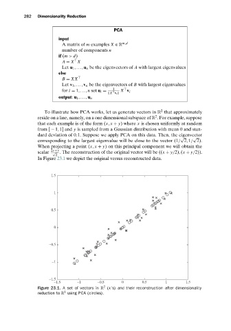
To illustrate how PCA works, let us generate vectors in R that approximately
2
reside on a line, namely, on a one dimensional subspace of R . For example, suppose
that each example is of the form (x,x + y)where x is chosen uniformly at random
from [ − 1,1] and y is sampled from a Gaussian distribution with mean 0 and stan-
dard deviation of 0.1. Suppose we apply PCA on this data. Then, the eigenvector
√ √
corresponding to the largest eigenvalue will be close to the vector (1/ 2,1/ 2).
When projecting a point (x,x + y) on this principal component we will obtain the
√ . The reconstruction of the original vector will be ((x + y/2),(x + y/2)).
scalar 2x+y
2
In Figure 23.1 we depict the original versus reconstructed data.

1.5

1

0.5

0

−0.5

−1

−1.5
−1.5 −1 −0.5 0 0.5 1 1.5
2
Figure 23.1. A set of vectors in R (x’s) and their reconstruction after dimensionality
1
reduction to R using PCA (circles).