Page 315 - Understanding Machine Learning

24. 1 M aximum Likelihood Estimator 297

As before, the maximum likelihood estimator is a maximizer of L( S;θ) with respect
to θ.
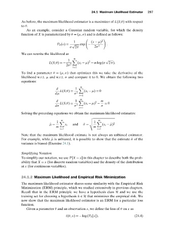
As an example, consider a Gaussian random variable, for which the density
function of X is parameterized by θ = (µ,σ) and is defined as follows:

1 ( x − µ) 2
P θ ( x) = √ exp − 2 .
σ 2π 2σ
We can rewrite the likelihood as
m
1 2 √

L( S;θ) =− 2 ( x i − µ) − m log(σ 2π).

2σ
i=1
To find a parameter θ = (µ,σ) that optimizes this we take the derivative of the
likelihood w.r.t. µ and w.r.t. σ and compare it to 0. We obtain the following two
equations:
m
d 1
L( S;θ) = ( x i − µ) = 0

dµ σ 2
i=1
m
d 1 2 m
L( S;θ) = ( x i − µ) − = 0

dσ σ 3 σ
i=1
Solving the preceding equations we obtain the maximum likelihood estimates:
4
m 5 m
1 5 1
ˆ µ = x i and ˆ σ = 6 ( x i − ˆµ) 2

m m
i=1 i=1
Note that the maximum likelihood estimate is not always an unbiased estimator.
For example, while ˆµ is unbiased, it is possible to show that the estimate ˆσ of the
variance is biased (Exercise 24.1).
Simplifying Notation
To simplify our notation, we use P[X = x] in this chapter to describe both the prob-
ability that X = x (for discrete random variables) and the density of the distribution
at x (for continuous variables).

24.1.2 Maximum Likelihood and Empirical Risk Minimization
The maximum likelihood estimator shares some similarity with the Empirical Risk
Minimization (ERM) principle, which we studied extensively in previous chapters.
Recall that in the ERM principle we have a hypothesis class H and we use the
training set for choosing a hypothesis h ∈ H that minimizes the empirical risk. We
now show that the maximum likelihood estimator is an ERM for a particular loss
function.
Given a parameter θ and an observation x, we define the loss of θ on x as

(θ,x) =−log(P θ [x]). (24.4)