Page 34 - Understanding Machine Learning

A Gentle Start
16

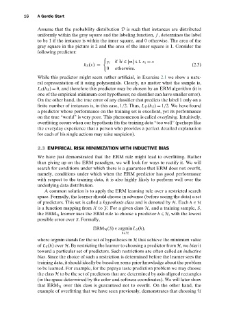
Assume that the probability distribution D is such that instances are distributed
uniformly within the gray square and the labeling function, f , determines the label
to be 1 if the instance is within the inner square, and 0 otherwise. The area of the
gray square in the picture is 2 and the area of the inner square is 1. Consider the
following predictor:

y i if ∃i ∈ [m]s.t. x i = x
h S (x) = (2.3)
0 otherwise.
o
t
c
i
fi
m
r

d
s

h
i
t
e
c
p
r

eem
a
r
h
er
a
t
g
h
i
i
t

s
r
t

e
w
s

e
s
2.1

ho
u
at
While this predictor mig ht seem rather artificia l, in Exercise 2.1 we show a natu--
W
n

w

a
i
,

i
h
a
il
l
n
r
c
xe
E
e
i

ral representation of it using polynomials. Clearly, no matter what the sample is,
L S (h S ) = 0, and therefore this predictor may be chosen by an ERM algorithm (it is
one of the empirical-minimum-cost hypotheses; no classifier can have smaller error).
On the other hand, the true error of any classifier that predicts the label 1 only on a

finite number of instances is, in this case, 1/2. Thus, L D (h S ) = 1/2. We have found

a predictor whose performance on the training set is excellent, yet its performance
on the true “world” is very poor. This phenomenon is called overfitting. Intuitively,
overfitting occurs when our hypothesis fits the training data “too well” (perhaps like
the everyday experience that a person who provides a perfect detailed explanation
for each of his single actions may raise suspicion).
2.3 EMPIRICAL RISK MINIMIZATION WITH INDUCTIVE BIAS
We have just demonstrated that the ERM rule might lead to overfitting. Rather
than giving up on the ERM paradigm, we will look for ways to rectify it. We will
search for conditions under which there is a guarantee that ERM does not overfit,
namely, conditions under which when the ERM predictor has good performance
with respect to the training data, it is also highly likely to perform well over the
underlying data distribution.
A common solution is to apply the ERM learning rule over a restricted search
space. Formally, the learner should choose in advance (before seeing the data) a set
of predictors. This set is called a hypothesis class and is denoted by H.Each h ∈ H
is a function mapping from X to Y. For a given class H, and a training sample, S,
the ERM H learner uses the ERM rule to choose a predictor h ∈ H, with the lowest
possible error over S. Formally,
ERM H (S) ∈ argmin L S (h),
h∈H
where argmin stands for the set of hypotheses in H that achieve the minimum value
of L S (h) over H. By restricting the learner to choosing a predictor from H,we bias it
toward a particular set of predictors. Such restrictions are often called an inductive
bias. Since the choice of such a restriction is determined before the learner sees the
training data, it should ideally be based on some prior knowledge about the problem
to be learned. For example, for the papaya taste prediction problem we may choose
the class H to be the set of predictors that are determined by axis aligned rectangles
(in the space determined by the color and softness coordinates). We will later show
that ERM H over this class is guaranteed not to overfit. On the other hand, the
example of overfitting that we have seen previously, demonstrates that choosing H