Page 45 - Understanding Machine Learning

3.2 A More General Learning Model 27

That is, we consider the expectation of the loss of h over objects z picked ran-
domly according to D. Similarly, we define the empirical risk to be the expected loss
m
over a given sample S = (z 1 ,...,z m ) ∈ Z , namely,
m
def 1
L S (h) = (h,z i ). (3.4)
m
i=1
The loss functions used in the preceding examples of classification and regression
tasks are as follows:

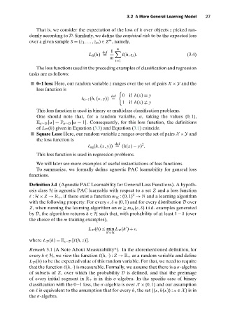
0–1 loss: Here, our random variable z ranges over the set of pairs X ×Y and the
loss function is

def 0 if h(x) = y
0−1 (h,(x, y)) =
1 if h(x) = y
This loss function is used in binary or multiclass classification problems.
One should note that, for a random variable, α, taking the values {0,1},
E α∼D [α] = P α∼D [α = 1]. Consequently, for this loss function, the definitions
of L D (h) given in Equation (3.3) and Equation (3.1) coincide.
Square Loss: Here, our random variable z ranges over the set of pairs X ×Y and
the loss function is
def 2
sq (h,(x, y)) = (h(x) − y) .
This loss function is used in regression problems.
We will later see more examples of useful instantiations of loss functions.
To summarize, we formally define agnostic PAC learnability for general loss
functions.

Definition 3.4 (Agnostic PAC Learnability for General Loss Functions). A hypoth-
esis class H is agnostic PAC learnable with respect to a set Z and a loss function
2
: H × Z → R + , if there exist a function m H :(0,1) → N and a learning algorithm
with the following property: For every
,δ ∈ (0,1) and for every distribution D over
Z, when running the learning algorithm on m ≥ m H (
,δ) i.i.d. examples generated
by D, the algorithm returns h ∈ H such that, with probability of at least 1 − δ (over
the choice of the m training examples),

L D (h) ≤ min L D (h ) +
,

h ∈H
where L D (h) = E z∼D [ (h,z)].
Remark 3.1 (A Note About Measurability*). In the aforementioned definition, for
every h ∈ H, we view the function (h,·): Z → R + as a random variable and define
L D (h) to be the expected value of this random variable. For that, we need to require
that the function (h,·) is measurable. Formally, we assume that there is a σ-algebra
of subsets of Z, over which the probability D is defined, and that the preimage
of every initial segment in R + is in this σ-algebra. In the specific case of binary
classification with the 0−1 loss, the σ-algebra is over X ×{0,1} and our assumption
on is equivalent to the assumption that for every h,the set {(x,h(x)) : x ∈ X} is in
the σ-algebra.