Page 56 - Understanding Machine Learning

The B ias-Complexity Tradeoff
38

That is, the probability to choose a pair ( x, y) is 1/|C| if the label y is indeed the true

( f i ) = 0.
label according to f i , and the probability is 0 if y = f i ( x). Clearly, L D i
We will show that for every algorithm, A, that receives a training set of m
examples from C × {0,1} and returns a function A( S) : C → {0,1}, it holds that
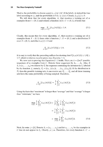
max E [ L D i ( A( S))] ≥ 1/4. (5.1)

i∈[ T ] S∼ D m
i
Clearly, this means that for every algorithm, A , that receives a training set of m

examples from X × {0,1} there exist a function f : X → {0,1} and a distribution D

over X × {0,1}, such that L D ( f ) = 0 and

E [ L D ( A ( S))] ≥ 1/4. (5.2)

m
S∼ D

It is easy to verify that the preceding suffices for showing that P[L D (A (S)) ≥ 1/8] ≥
1/7, which is what we need to prove (see Exercise 5.1).
m
We now turn to proving that Equation (5.1) holds. There are k = (2m) possible
sequences of m examples from C. Denote these sequences by S 1 ,..., S k . Also, if
i
S j = (x 1 ,...,x m ) we denote by S the sequence containing the instances in S j labeled
j
i
by the function f i , namely, S = ((x 1 , f i (x 1 )),...,(x m , f i (x m ))). If the distribution is
j
i
i
D i then the possible training sets A can receive are S ,..., S , and all these training
1 k
sets have the same probability of being sampled. Therefore,
k
1 i
(A(S))] = (A(S )). (5.3)
E [L D i L D i j
m
S∼D i k
j=1
Using the facts that “maximum” is larger than “average” and that “average” is larger
than “minimum,” we have
k T k
1 i 1 1 i
max L D i (A(S )) ≥ L D i (A(S ))
j
j
i∈[T] k T k
j=1 i=1 j=1
k T
1 1 i
= L D i (A(S ))
j
k T
j=1 i=1
T
1 i
≥ min L D i (A(S )). (5.4)
j
j∈[k] T
i=1
Next, fix some j ∈ [k]. Denote S j = (x 1 ,...,x m )and let v 1 ,...,v p be the examples in
C that do not appear in S j . Clearly, p ≥ m. Therefore, for every function h : C →