Page 62 - Understanding Machine Learning

The VC-Dimension
44

Example 6.1. Let H be the set of threshold functions over the real line, namely,
H ={h a : a ∈ R},where h a : R →{0,1} is a function such that h a (x) = 1 [x<a] .To
remind the reader, 1 [x<a] is 1 if x < a and 0 otherwise. Clearly, H is of infinite size.
Nevertheless, the following lemma shows that H is learnable in the PAC model
using the ERM algorithm.
Lemma 6.1. Let H be the class of thresholds as defined earlier. Then, H is PAC
learnable, using the ERM rule, with sample complexity of m H(
,δ) ≤ log(2/δ)/
.

Proof. Let a be a threshold such that the hypothesis h (x) = 1 [x<a ] achieves

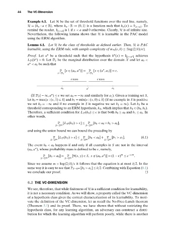
L D (h ) = 0. Let D x be the marginal distribution over the domain X and let a 0 <

a < a 1 be such that

P [x ∈ (a 0 ,a )] = P [x ∈ (a ,a 1 )] =
.
x∼D x x∼D x
ε mass ε mass
a 0 a * a 1

(If D x ( − ,a ) ≤
we set a 0 =−∞ and similarly for a 1 ). Given a training set S,
let b 0 = max{x :(x,1) ∈ S} and b 1 = min{x :(x,0) ∈ S} (if no example in S is positive
we set b 0 =−∞ and if no example in S is negative we set b 1 =∞). Let b S be a
threshold corresponding to an ERM hypothesis, h S , which implies that b S ∈ (b 0 ,b 1 ).
Therefore, a sufficient condition for L D (h S ) ≤
is that both b 0 ≥ a 0 and b 1 ≤ a 1 .In
other words,
P [L D (h S ) >
] ≤ P [b 0 < a 0 ∨ b 1 > a 1 ],
m m
S∼D S∼D
and using the union bound we can bound the preceding by

P [L D (h S ) >
] ≤ P [b 0 < a 0 ] + P [b 1 > a 1 ]. (6.1)
S∼D m S∼D m S∼D m
The event b 0 < a 0 happens if and only if all examples in S are not in the interval
(a 0 ,a ), whose probability mass is defined to be
, namely,
∗
m

P [b 0 < a 0 ] = P [∀(x, y) ∈ S, x ∈ (a 0 ,a )] = (1 −
) ≤ e −
m .
S∼D m S∼D m
Since we assume m > log(2/δ)/
it follows that the equation is at most δ/2. In the
same way it is easy to see that P S∼D [b 1 > a 1 ] ≤ δ/2. Combining with Equation (6.1)
m
we conclude our proof.

6.2 THE VC-DIMENSION

We see, therefore, that while finiteness of H is a sufficient condition for learnability,
it is not a necessary condition. As we will show, a property called the VC-dimension
of a hypothesis class gives the correct characterization of its learnability. To moti-
vate the definition of the VC-dimension, let us recall the No-Free-Lunch theorem
(Theorem 5.1) and its proof. There, we have shown that without restricting the
hypothesis class, for any learning algorithm, an adversary can construct a distri-
bution for which the learning algorithm will perform poorly, while there is another