Page 121 - ISCI’2017

∞
er ∫
P = ϕ ∆ P )d∆ . (65)
( ) ( , λ ∆
0

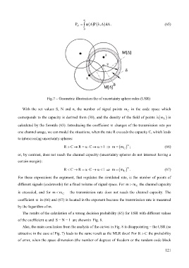
Fig.7 – Geometric illustration the of uncertainty sphere rules (USR)

With the set values S, N and n, the number of signal points m C in the code space which

corresponds to the capacity is derived from (30), and the density of the field of points (mλ C ) is

calculated by the formula (63). Introducing the coefficient α changes of the transmission rate per

one channel usage, we can model the situations, when the rate R exceeds the capacity C, which leads
to intercrossing uncertainty spheres:

C
R > C → R = α⋅ → α > 1 ⇒ m = (m C ) α ; (66)

or, by contrast, does not reach the channel capacity (uncertainty spheres do not intersect having a
certain margin):

R < C → R = α⋅ → α < 1 ⇒ m = (m C ) α . (67)
C
For these expressions the argument, that regulates the simulated rate, is the number of points of
different signals (codewords) for a fixed volume of signal space. For m > m C the channel capacity

is exceeded, and for m < m C – the transmission rate does not reach the channel capacity. The

coefficient in (66) and (67) is located in the exponent because the transmission rate is measured
α
by the logarithm of m.

The results of the calculation of a wrong decision probability (65) for USR with different values
of the coefficient α and S = N = 1 are shownin Fig. 8.

Alas, the main conclusion from the analysis of the curves in Fig. 8 is disappointing – the USR (so

attractive in the case of Fig. 7) leads to the same result as the MLR does! For R > C the probability
of error, when the space dimension (the number of degrees of freedom or the random code block

121