Page 7 - Tourism Flows Prediction based on an Improved Grey GM(1,1) Model

Xiangyun Liu et al. / Procedia - Social and Behavioral Sciences 138 ( 2014 ) 767 – 775 773
1564 k
x 1 k 1 273239 54739e 0 5 105910 74739 (18)
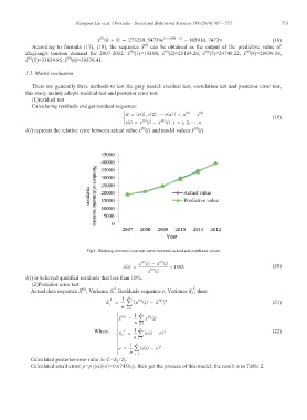
According to formula (17), (18), the sequence x ̑ (0) can be obtained as the output of the predictive value of
Zhejiang's tourism demand for 2007-2012. x ̑ (0) (1)=19100, x ̑ (0) (2)=21164.20, x ̑ (0) (3)=24748.22, x ̑ (0) (4)=28939.18,
x ̑ (0) (5)=33839.85, x ̑ (0) (6)=39570.41.

5.2. Model evaluation
There are generally three methods to test the gray model: residual test, correlation test and posterior error test,
this study mainly adopts residual test and posterior error test.
(1)residual test
Calculating residuals and get residual sequence:
­ e 1 e 2 " e n x 0 x 0
°E
® (19)
0
0

¯
° ie x i x i i 21 " n
(0)
δ(i) reprents the relative error between actual value x (i) and model values x ̑ (0) (i).

Fig.1. Zhejiang domestic tourism curve between actual and predicted values
0
x 0 (i x i
G i u 100 (20)
x 0 i
δ(i) is believed qualified residuals that less than 10%.
(2)Posterior error test
2
2
(0)
Actual data sequence X , Variance S 1 , Residuals sequence e, Variance S 2 , then:
2 1 n 0 0 2
S ¦ x i x (21)
1
n i 1
­ 0 1 n 0
° x ¦ x i
° n i 1
1
n
Where ° 2 ¦ e i e 2 (22)
® S
° 2 n i 1
° 1 n
°e ¦ e i e 2
¯ n i 1
Calculated posterior error ratio is: C=S 2 ⁄ S 1 .
Calculated small error: p=p{|e(i)-ē|<0.6745S 1 }, then get the process of this model; the result is in Table 2.