Page 52 - Clinical Small Animal Internal Medicine

20 Section 1 Evaluation and Management of the Patient

takes for an estimated 50% probability of patients to die (obtained by dividing the number of deaths [6] by the
VetBooks.ir is called the median survival time. In the above example, total amount of time all patients spent alive and at risk of
dying [72 years]). Although this number is admittedly
the median time to death is seven years. With larger
datasets, it would also be achievable to estimate the
a fractional death, it is better understood when invento-
time it would take for a 10%, 25%, 75%, 95%, etc. proba- difficult to understand because it is not possible to have
bility of death. rying multiple years as a patient: 8.3 deaths for every 100
In the less common case that patients are followed for patient‐years alive, six deaths for every 72 patient‐years
identical periods of time, or inferences are restricted to alive, etc.
briefer periods that most or all patients were followed Using rate information is invaluable in assessing the
through, it becomes possible to estimate the risk of out- course of a health outcome because it is possible for the
comes for such time periods, either unconditionally or probability of the outcome to be the same across groups
conditional on possible determinants of the outcomes. for the same amount of follow‐up, even while the rates of
For example, the one‐year risk of death from patients the outcome occurring are different. To illustrate this,
diagnosed with IMHA conditional on sex can be calcu- consider two drugs (drug A and drug B) used to cure a
lated, and expressed (typically) as a risk ratio (sometimes particular disease, both of which are 100% effective.
referred to as a relative risk). It is conventional to report However, drug A cures the disease much faster than drug
ratio statistics accompanied by: (1) their respective 95% B, making drug A more desirable than drug B (ignoring
confidence intervals to demonstrate the degree of preci- other relevant issues such as cost, side‐effects, etc.). This
sion associated with the statistic, and (2) P‐values corre- is equivalent to saying that the rate of cure under drug A
sponding to a test of the null hypothesis that the risk is higher than the rate of cure under drug B.
ratio = 1 (i.e., there is no difference in the risks of the We can assign hypothetical numbers to further the
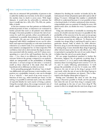
outcome between the groups compared in an analysis), discussion. Suppose the six patients receiving drug A
which are interpretable as the probabilities of finding were cured at 1, 2, 3, 4, 5, and 6 weeks following admin-
risk ratios >1 at least as large (or risk ratios <1 at least as istration; those receiving drug B were cured at 7, 8, 9, 10,
small) as those observed in the study when the null 11, and 12 weeks following administration. In both
hypothesis (of no difference in risks) is correct. groups the probability of cure by 12 weeks was 100%.
In the preceding paragraph, the phrase “rate of death” However, the rate of cure in the drug A group is 0.29
was deliberately not used because a rate is neither a pro- case/week, while the rate of cure in the drug B group is
portion nor a probability. Instead, a rate can be thought 0.11 case/week (calculations not shown). This is illus-
of as a “velocity” – how much of an event occurs as a trated in the Kaplan–Meier plot in Figure 3.1.
function of time (e.g., miles traveled per hour). In this Having now calculated the rates of cure (by drug
setting, it is possible to estimate such a rate: the number group), it becomes possible to finally ask the question:
of expected deaths for each year(s) of being a patient. how does the rate of cure from drug A compare (rela-
Using the example above, the average (constant) rate of tively speaking) to the rate of cure from drug B? The
death equals 0.0833 death/patient‐year as a patient answer to this is to simply take the rate from drug A and

1.00 Figure 3.1 Rate of cure illustrated in a Kaplan–
Meier plot.

Probability of being diseased 0.50
0.75

0.25

0.00
0 5 10 15
Time (weeks)
Drug A Drug B