Page 172 - Six Sigma Advanced Tools for Black Belts and Master Black Belts

OTE/SPH
OTE/SPH
2:57
August 31, 2006
Char Count= 0
JWBK119-11
Empirical Distribution Function based Approaches 157
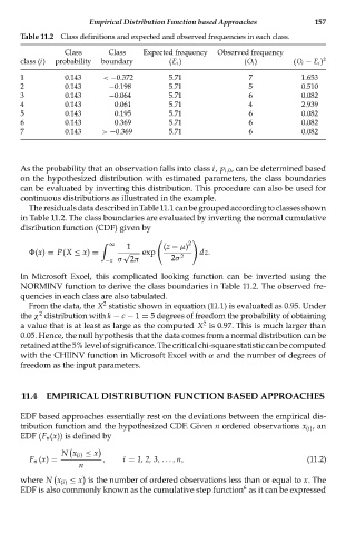
Table 11.2 Class definitions and expected and observed frequencies in each class.
Class Class Expected frequency Observed frequency
class (i) probability boundary (E i ) (O i ) (O i − E i ) 2
1 0.143 < −0.372 5.71 7 1.653
2 0.143 −0.198 5.71 5 0.510
3 0.143 −0.064 5.71 6 0.082
4 0.143 0.061 5.71 4 2.939
5 0.143 0.195 5.71 6 0.082
6 0.143 0.369 5.71 6 0.082
7 0.143 > −0.369 5.71 6 0.082

As the probability that an observation falls into class i, p i,0 , can be determined based
on the hypothesized distribution with estimated parameters, the class boundaries
can be evaluated by inverting this distribution. This procedure can also be used for
continuous distributions as illustrated in the example.
TheresidualsdatadescribedinTable11.1canbegroupedaccordingtoclassesshown
in Table 11.2. The class boundaries are evaluated by inverting the normal cumulative
disribution function (CDF) given by

1 (z − μ)
∞
2
(x) = P(X ≤ x) = √ exp 2 dz.
−x σ 2π 2σ
In Microsoft Excel, this complicated looking function can be inverted using the
NORMINV function to derive the class boundaries in Table 11.2. The observed fre-
quencies in each class are also tabulated.
2
From the data, the X statistic shown in equation (11.1) is evaluated as 0.95. Under
2
the χ distribution with k − c − 1 = 5 degrees of freedom the probability of obtaining
2
a value that is at least as large as the computed X is 0.97. This is much larger than
0.05. Hence, the null hypothesis that the data comes from a normal distribution can be
retainedatthe5%levelofsignificance.Thecriticalchi-squarestatisticcanbecomputed
with the CHIINV function in Microsoft Excel with α and the number of degrees of
freedom as the input parameters.

11.4 EMPIRICAL DISTRIBUTION FUNCTION BASED APPROACHES

EDF based approaches essentially rest on the deviations between the empirical dis-
tribution function and the hypothesized CDF. Given n ordered observations x (i) ,an
EDF (F n (x)) is defined by

N x (i) ≤ x
F n (x) = , i = 1, 2, 3,..., n, (11.2)
n

where N x (i) ≤ x is the number of ordered observations less than or equal to x. The

6
EDF is also commonly known as the cumulative step function as it can be expressed