Page 374 - Maxwell House

354 Chapter 7

The open question is what strategy we can use when there are several discontinuities in the
same line. If they are located so close that their reactive near-fields are overlapped, the only
valuable option is a numerical approach. However, in many or maybe most practical cases the
local discontinuities are separated far enough in term of wavelength meaning that all nearby
evanescent (exponentially decaying) modes practically extinct. Then the lone dominant mode
supports all the interactions between discontinuities. Keeping it in mind, we will describe two
tactics by the end of this chapter. One is graphical and based on so-called lattice diagram
somehow similar to phasor diagram we have used in Chapter 5. Another one is the general
algorithm lets solve this problem more formally and for a much wider set of challenges. This
algorithm operates with scattering matrices describing the behavior of each discontinuity.
As we have shown in the previous chapter, the vast variety of different feed lines are in practical
use. Despite it, the set of discontinues in all of them is nearly the same, the realization is
different. Therefore, it is quite attractive and sufficient to study one type of line and then discuss
some possible adjustments if the line is changed. For several reasons, we chose the coaxial line
as a model. First, the dominant mode in this line is frequency independent TEM-mode. It
impressively simplifies and accelerates the EM analysis and the following development of
equivalent transmission line circuitry. There are no troubles with the line characteristic
impedance; it can be defined uniquely. The frequency gap between the cut-off frequencies of
the dominant and the first higher mode is wide enough (several octaves, for example) that makes
possible an extremely broadband single mode simulation.

7.1 COAXIAL DISCONTINUES
7.1.1 Dielectric Beads Supporting Center Conductor

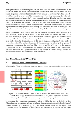
The complete filling of the internal space between the center and outer conductors sometimes

Figure 7.1.1 Coaxial cable with periodic beads: a) Schematic, b) Cascade connection, c)
E- and H-field energy distribution around and inside single bead, d) Equivalent circuit
with lump elements, e) Smith chart for single bead showing capacitance impedance

is not desired due to an extra attenuation and weight, vanishing the required flexibility of line,
fabrication cost, etc. Alternatively, we can place a discrete supporting set of dielectric beads of
relative permittivity (typically, = 1) and width w in the distance d, as Figure 7.1.1a

illustrates. From the definition of the characteristic impedance of coaxial line we know