Page 110 - Mechatronics with Experiments

96 MECHATRONICS
20 log ⏐G⏐ 20 log ⏐G⏐
10 10
40 40
20 20
0 0
–2 –1 0 1 2 log ω –2 –1 0 1 2 log ω
10
10
–20 –20
0.01 0.1 1 10 100 0.01 0.1 1 10 100
–40 –40 ω = K
1 V
20 log ⏐G⏐
10

log ω
10

ω 2
K = ω 2
a 2
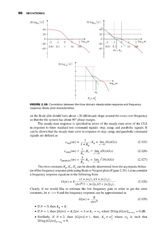
FIGURE 2.39: Correlation between the time domain steady-state response and frequency
response (Bode plot) characteristics.

on the Bode plot should have about −20 dB/decade slope around the cross-over frequency
◦
so that the the system has about 90 phase margin.
The steady-state response is specified in terms of the steady-state error of the CLS
in response to three standard test command signals: step, ramp, and parabolic signals. It
can be shown that the steady-state error in response to step, ramp, and parabolic command
signals are defined as
1
e (∞) = ; K = lim D(s)G(s) (2.125)
step p
1 + K p s⟶0
1
e ramp (∞) = ; K = lim sD(s)G(s) (2.126)
v
K v s⟶0
1 2
e parabolic (∞) = ; K = lim s D(s)G(s) (2.127)
a
K a s⟶0
The error constants K , K , K can be directly determined from the asymptotic behav-
p v a
ior of the frequency response plots using Bode or Nyquist plots (Figure 2.39). Let us consider
a frequency response equation in the following form
(1 + jw∕z )(1 + jw∕z )...
1
2
G(jw) = K (2.128)
(jw) (1 + jw∕p )(1 + jw∕p )...
N
1 2
Clearly, if we would like to estimate the low frequency gain in order to get the error
constants, let w ⟶ 0 and the frequency response can be approximated as
K
G(jw) ≈ (2.129)
(jw) N
If N = 0, then K = K.

p
= 0dB.
1
v
If N = 1, then |G(jw)| = K∕|jw| = 1or K = w where 20 log |G(jw)| w=w 1
Similarly, If N = 2, then |G(jw)| = 1, then, K = w 2 where w 2 is such that
2
a
= 0.
20 log |G(jw)|
w=w 2