Page 841 - Mechatronics with Experiments

®
®
MATLAB , SIMULINK , STATEFLOW, AND AUTO-CODE GENERATION 827
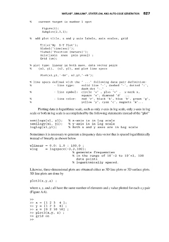
% current target is number 1 spot
Figure(1);
Subplot(2,3,1);
% add plot title, x and y axis labels, axis scales, grid

Title(’My X-Y Plot’);
Xlabel(’time(sec)’);
Ylabel(’Position (meters)’);
Axis([xmin xmax ymin ymax]) ;
Grid (on);
% plot type: linear in both axes, data vector pairs
% (x1, y1), (x2, y2), and plot line specs
Plot(x1,y1,’-0r’, x2,y2,’–+b’);

% line specs defined with the ’ ...’ following data pair definition:
% - line type: solid line ’-’, dashed ’–’, dotted ’:’,
dash-dot ’-.’ ...
% - line symbol: circle ’o’ , plus ’+’ , x-mark x,
square ’s’, diamond ’d’ ...
% - line color: red ’r’, black ’k’, blue ’b’, green ’g’,
% yellow ’y’, cyan ’c’, magneta ’m’...

Plotting data in logarithmic scale, such as only x-axis in log scale, only y-axis in log
scale or both in log scale is accomplished by the following statements instead of the “plot”

semilogx(x1, y1); % x-axis is in Log scale
semilogy(x1, y1); % y-axis is in Log scale
loglog(x1,y1); % Both x and y axes are in Log scale

Sometimes it is necessary to generate a frequency data vector that is spaced logarithmically
instead of linearly as shown below

wlinear = 0.0: 1.0 : 100.0 ;
wlog = logspace(-3,3,100);
% generate frequencies
% in the range of 10ˆ-3 to 10ˆ+3, 100
data points
% logaritmically spaced.
Likewise, three-dimensional plots are obtained either as 3D line plots or 3D surface plots.
3D line plots are done by
plot3(x,y,z) ;

where x, y, and z all have the same number of elements and z value plotted for each x,y pair
(Figure A.6).

>>
>> x = [1 2 3 4 ];
>> y = [1 2 3 4] ;
>> z = [0 2 10 50] ;
>> plot3(x,y, z) ;
>> grid on
>>