Page 843 - Mechatronics with Experiments

®
®
MATLAB , SIMULINK , STATEFLOW, AND AUTO-CODE GENERATION 829
Y =

-1.0000 -1.0000 -1.0000 -1.0000 -1.0000
-0.5000 -0.5000 -0.5000 -0.5000 -0.5000
0 0 0 0 0
0.5000 0.5000 0.5000 0.5000 0.5000
1.0000 1.0000 1.0000 1.0000 1.0000

Z =
-0.1353 -0.1433 0 0.1433 0.1353
-0.2865 -0.3033 0 0.3033 0.2865
-0.3679 -0.3894 0 0.3894 0.3679
-0.2865 -0.3033 0 0.3033 0.2865
-0.1353 -0.1433 0 0.1433 0.1353
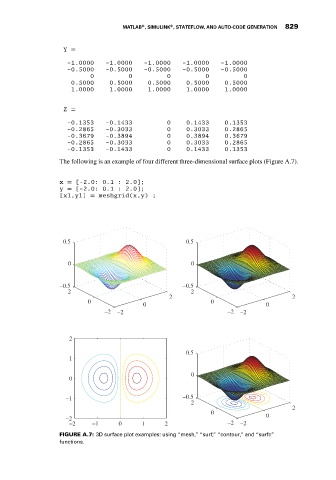
The following is an example of four different three-dimensional surface plots (Figure A.7).

x = [-2.0: 0.1 : 2.0];
y = [-2.0: 0.1 : 2.0];
[x1,y1] = meshgrid(x,y) ;

0.5 0.5

0 0

−0.5 −0.5
2 2
2 2
0 0
0 0
−2 −2 −2 −2

2

0.5
1

0
0

−1 −0.5
2
2
0 0
−2
−2 −1 0 1 2 −2 −2
FIGURE A.7: 3D surface plot examples: using “mesh,” “surf,” “contour,” and “surfc”
functions.