Page 847 - Mechatronics with Experiments

®
®
MATLAB , SIMULINK , STATEFLOW, AND AUTO-CODE GENERATION 833
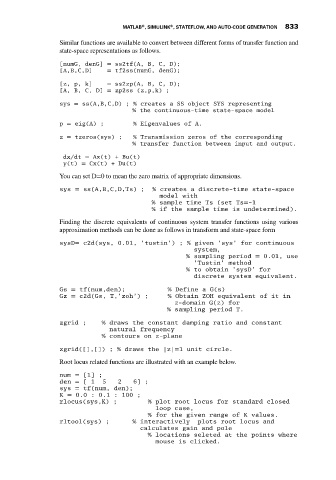
Similar functions are available to convert between different forms of transfer function and
state-space representations as follows.
[numG, denG] = ss2tf(A, B, C, D);
[A,B,C,D] = tf2ss(numG, denG);

[z, p, k] = ss2zp(A, B, C, D);
[A, B, C, D] = zp2ss (z,p,k) ;
sys = ss(A,B,C,D) ; % creates a SS object SYS representing
% the continuous-time state-space model
p = eig(A) ; % Eigenvalues of A.

z = tzeros(sys) ; % Transmission zeros of the corresponding
% transfer function between input and output.
dx/dt = Ax(t) + Bu(t)
y(t) = Cx(t) + Du(t)
You can set D=0 to mean the zero matrix of appropriate dimensions.
sys = ss(A,B,C,D,Ts) ; % creates a discrete-time state-space
model with
% sample time Ts (set Ts=-1
% if the sample time is undetermined).

Finding the discrete equivalents of continuous system transfer functions using various
approximation methods can be done as follows in transform and state-space form

sysD= c2d(sys, 0.01, ’tustin’) ; % given ’sys’ for continuous
system,
% sampling period = 0.01, use
’Tustin’ method
% to obtain ’sysD’ for
discrete system equivalent.
Gs = tf(num,den); % Define a G(s)
Gz = c2d(Gs, T,’zoh’) ; % Obtain ZOH equivalent of it in
z-domain G(z) for
% sampling period T.

zgrid ; % draws the constant damping ratio and constant
natural frequency
% contours on z-plane
zgrid([],[]) ; % draws the |z|=1 unit circle.

Root locus related functions are illustrated with an example below.
num = [1] ;
den = [ 1 5 2 6] ;
sys = tf(num, den);
K = 0.0 : 0.1 : 100 ;
rlocus(sys,K) ; % plot root locus for standard closed
loop case,
% for the given range of K values.
rltool(sys) ; % interactively plots root locus and
calculates gain and pole
% locations seleted at the points where
mouse is clicked.