Page 883 - Mechatronics with Experiments

®
®
MATLAB , SIMULINK , STATEFLOW, AND AUTO-CODE GENERATION 869

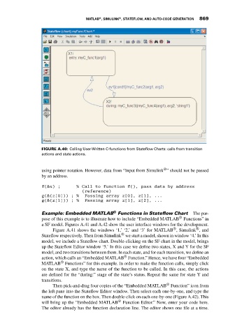
FIGURE A.40: Calling User-Written C-functions from Stateflow Charts: calls from transition
actions and state actions.

®
using pointer notation. However, data from “Input from Simulink ” should not be passed
by an address.

f(&x) ; % Call to function f(), pass data by address
(reference)
g(&(z[0])) ; % Passing array z[0], z[1], ...
g(&(z[1])) ; % Passing array z[1], z[2], ...

®
Example: Embedded MATLAB Functions in Stateflow Chart The pur-
®
pose of this example is to illustrate how to include “Embedded MATLAB Functions” in
a SF model. Figures A.41 and A.42 show the user interface windows for the development.
®
®
Figure A.41 shows the windows ‘1,’ ‘2,’ and ‘3’ for MATLAB , Simulink , and
®
Stateflow respectively. Then from Simulink we start a model, shown in window ‘4.’ In this
model, we include a Stateflow chart. Double-clicking on the SF chart in the model, brings
up the Stateflow Editor window ‘5.’ In this case we define two states, X and Y for the SF
model, and two transitions between them. In each state, and for each transition, we define an
®
action, which calls an “Embedded MATLAB Function.” Hence, we have four “Embedded
®
MATLAB Functions” for this example. In order to make the function calls, simply click
on the state X, and type the name of the function to be called. In this case, the actions
are defined for the “during:” stage of the state’s status. Repeat the same for state Y and
transitions.
®
Then pick-and-drag four copies of the “Embedded MATLAB Function” icon from
the left pane into the Stateflow Editor window. Then select each one-by-one, and type the
name of the function on the box. Then double-click on each one-by-one (Figure A.42). This
will bring up the “Embedded MATLAB ® Function Editor.” Now, enter your code here.
The editor already has the function declaration line. The editor shows one file at a time.