Page 3 - The $ game .dvi

J. Vitting Andersen and D. Sornette: The $-game 143

500 to zero [10]. As shown in [15], this can be achieved by the
following generalization of (2):
MG−payoff −500 r(t) ≡ ln(p(t)) − ln(p(t − 1)) = (A(t) − S M (t))/λ, (5)
0

−1000 t−1
with S M (t)= − A(t). Expression (5) implies that,
t=0
the larger is the long position the market-maker is holding,
−1500
0 50 100 150 200 250 300 350 400 450 500
t the more he will lower the price in order to attract buyers,
and vice versa for a short position. Another way to ensure
the same behavior is to introduce a spread or change the
1.5
1 available liquidity [17].
MG−wealth −0.5 0 ing from a market competition between agents with payoff
0.5
We first study the price formation using (2) and result-
−1
case with no constraint on the number of stocks held by
−1.5 function (3) and compare it with the MG case (1) in the
−2 each agent (i.e., anagent canopena newpositionateach
0 50 100 150 200 250 300 350 400 450 500
t time step). Contrary to the MG case, we find that the
price always diverges to infinity or goes zero within a few
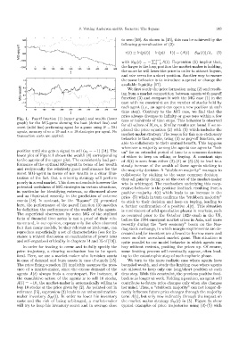
Fig. 1. Payoff function (1) (upper graph) and wealth (lower
tens or hundreds of time steps. This behavior is observed
graph) for the MG-game showing the best (dotted line) and
for all values of N, m, s. Similar results are found if we re-
worst (solid line) performing agent for a game using N = 501
agents, memory of m =10 and s = 10 strategies per agent. No placed the price equation (2) with (5) which includes the
market-maker strategy. The reason for this non-stationary
transaction costs are applied.
behavior is that agents, using (3) as pay-off function, are
able to collaborate to their mutual benefit. This happens
whenever a majority among the agents can agree to “lock
position until she gets a signal to sell (a i = −1) [14]. The on” for an extended period of time to a common decision
lower plot of Figure 1 shows the wealth (4) corresponding of either to keep on selling or buying. A constant sign
to the agents of the upper plot. The consistently bad per- of A(t) is seen from either (2)-(4) or (3)-(5) to lead to a
formance of the optimal MG-agent in terms of her wealth steady increase of the wealth of those agents sticking to
and reciprocally the relatively good performance for the the majority decision. A “stubborn majority” manages to
worst MG-agent in terms of her wealth is a clear illus- collaborate by sticking to the same common decision –
tration of the fact that a minority strategy will perform they all gain by doing so at the cost of the market-maker
poorly in a real market. This does not exclude however the who is arbitraged. The mechanism underlying this coop-
potential usefulness of MG strategies in certain situations, erative behavior is the positive feedback resulting from a
in particular for identifying extrema, as discussed above positive majority A(t) which leads to an increase in the
and as illustrated recently in the prediction of extreme price (5) which in turn confirms the “stubborn majority”
events [18]. In contrast, for the “$-game” (3) presented to stick to their decision and keep on buying, leading to
here, the performance of the payoff function (3) matches a further confirmation of a positive A(t). This situation
by definition the performance of the wealth of the agents. is reminiscent of wild speculative phases in markets, such
The superficial observance by some MG of the stylized as occurred prior to the October 1929 crash in the US,
facts of financial time series is not a proof of their rele- before the 1994 emergent market crises in Asia, and more
vance and, in our opinion, express only the often observed recently during the “new economy” boom on the Nas-
fact that many models, be they relevant or irrelevant, can daq stock exchange, in which margin requirements are de-
reproduce superficially a set of characteristics (see for in- creased and/or investors are allowed to borrow more and
stance a related discussion on mechanisms of power laws more on their unrealized market gains. This situation is
and self-organized criticality in chapters 14 and 15 of [19]). quite parallel to our model behavior in which agents can
In order for trading to occur and to fully specify the buy without restrain, pushing the prices up. Of course,
price trajectory, a clearing mechanism has to be speci- some limiting process will eventually appear, often lead-
ficed. Here, we use a market maker who furnishes assets ing to the catastrophic stop of such euphoric phase.
in case of demand and buys assets in case of supply [15]. We turn to the more realistic case where agents have
The price fixing equation (2) implicitly assumes the pres- bounded wealth, and study the limiting case where agents
ence of a market-maker, since the excess demand of the are allowed to keep only one long/short position at each
agents A(t) always finds a counterpart. For instance, if time step. With this constraint, the previous positive feed-
the cumulative action of the agents is to sell 10 stocks, back is no longer at work. Holding a position, an agent will
A(t)= −10, the market-maker is automatically willing to contribute to future price changes only when she changes
buy 10 stocks at the price given by (2). As pointed out in her mind. Thus, a “stubborn majority” can not longer di-
reference [15], expression (2) leads to an unbound market- rectly influence future price changes through the majority
maker inventory S M (t). In order to lower his inventory term A(t), but only now indirectly through the impact on
costs and the risk of being arbitraged, a market-maker the market maker strategy S M (t) in (5). Figure 2a show
will try to keep his inventory secret and in average close typical examples of price trajectories using (3)-(5) with