Page 9 - DOC-20220324-WA0012.-488-500

11.1 Methods for First-Order Systems 473

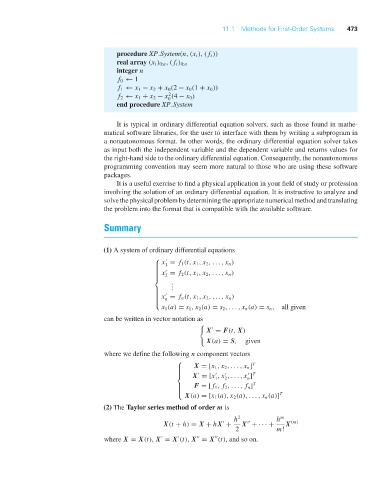
procedure XP System(n,(x i ), ( f i ))
real array (x i ) 0:n ,( f i ) 0:n
integer n
f 0 ← 1
f 1 ← x 1 − x 2 + x 0 (2 − x 0 (1 + x 0 ))
2
f 2 ← x 1 + x 2 − x (4 − x 0 )
0
end procedure XP System

It is typical in ordinary differential equation solvers, such as those found in mathe-
matical software libraries, for the user to interface with them by writing a subprogram in
a nonautonomous format. In other words, the ordinary differential equation solver takes
as input both the independent variable and the dependent variable and returns values for
the right-hand side to the ordinary differential equation. Consequently, the nonautonomous
programming convention may seem more natural to those who are using these software
packages.
It is a useful exercise to find a physical application in your field of study or profession
involving the solution of an ordinary differential equation. It is instructive to analyze and
solve the physical problem by determining the appropriate numerical method and translating
the problem into the format that is compatible with the available software.

Summary

(1) A system of ordinary differential equations
⎧
x = f 1 (t, x 1 , x 2 ,..., x n )
⎪ 1
⎪
⎪

⎪ x = f 2 (t, x 1 , x 2 ,..., x n )
⎪
⎪ 2
⎨
.
.
⎪ .
⎪

⎪ x = f n (t, x 1 , x 2 ,..., x n )
⎪
⎪ n
⎪
⎩
x 1 (a) = s 1 , x 2 (a) = s 2 ,..., x n (a) = s n , all given
can be written in vector notation as

X = F(t, X)

X(a) = S, given
where we define the following n component vectors
⎧
X = [x 1 , x 2 ,..., x n ] T
⎪
⎪
⎪
X = [x , x ,..., x ]
⎨ T
n
2
1
F = [ f 1 , f 2 ,..., f n ] T
⎪
⎪
⎪
⎩ T
X(a) = [x 1 (a), x 2 (a),..., x n (a)]
(2) The Taylor series method of order m is
h 2 h m
(m)
X(t + h) = X + hX + X + ··· + X
2 m!

where X = X(t), X = X (t), X = X (t), and so on.