Page 7 - DOC-20220324-WA0012.-488-500

11.1 Methods for First-Order Systems 471

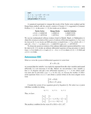
real t
f 1 ← x 1 − x 2 + t(2 − t(1 + t))
2
f 2 ← x 1 + x 2 − t (4 − t)
end procedure XP System

A numerical experiment to compare the results of the Taylor series method and the
Runge-Kutta method with the analytic solution of System (1) is suggested in Computer
Problem 11.1.1. At the point t = 1.0, the results are as follows:

Taylor Series Runge-Kutta Analytic Solution
x(1.0) ≈ 2.46869 40 2.46869 42 2.46869 39399
y(1.0) ≈ 1.28735 46 1.28735 61 1.28735 52872
We can use mathematical software routines found in Matlab, Maple, or Mathematica to
obtain the numerical solution of the system of ordinary differential equations (1). For t over
the interval [0, 1], we invoke an ODE procedure to march from t = 0 at which x(0) = 1
and y(0) = 0to t = 1 at which x(1) = 2.468693912 and y(1) = 1.287355325.
To obtain the numerical solution of the ordinary differential equation defined for t over
the interval [1, 1.5], invoke an ordinary differential equation solving procedure to march
from t = 0 at which x(1) = 2 and y(1) =−2to t = 1.5 at which x(1.5) ≈ 15.5028 and
y(1.5) ≈ 6.15486.

Autonomous ODE
When we wrote the system of differential equations in vector form

X = F(t, X)
we assumed that the variable t was explicitly separated from the other variables and treated
differently. It is not necessary to do this. Indeed, we can introduce a new variable x 0
that is t in disguise and add a new differential equation x = 1. A new initial condi-

0
tion must also be provided, x 0 (a) = a. In this way, we increase the number of differ-
ential equations from n to n + 1 and obtain a system written in the more elegant vector
form

X = F(X)
X(a) = S, given
Consider the system of two equations given by Equation (1). We write it as a system
with three variables by letting

x 0 = t, x 1 = x, x 2 = y
Thus, we have
⎡ ⎤ ⎡ ⎤
x 1
0
⎢ ⎥ ⎢ 2 3 ⎥
0
0
1
⎣ x ⎦ = ⎣ x 1 − x 2 + 2x 0 − x − x ⎦
2
x x 1 + x 2 − 4x + x 3
2 0 0
T
The auxiliary condition for the vector X is X(0) = [0, 1, 0] .