Page 204 - Krugmans Economics for AP Text Book_Neat

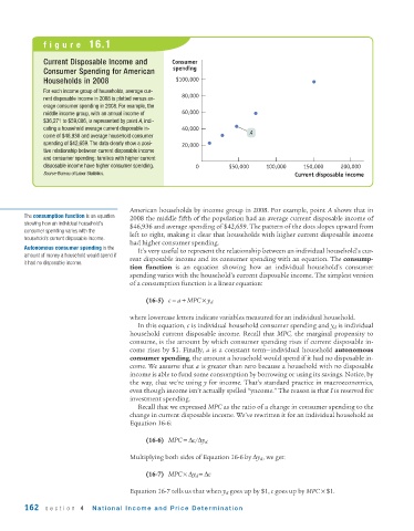
figure 16.1

Current Disposable Income and Consumer
spending
Consumer Spending for American
Households in 2008 $100,000
For each income group of households, average cur-
80,000
rent disposable income in 2008 is plotted versus av-
erage consumer spending in 2008. For example, the
middle income group, with an annual income of 60,000
$36,271 to $59,086, is represented by point A, indi-
cating a household average current disposable in- 40,000
A
come of $46,936 and average household consumer
spending of $42,659. The data clearly show a posi- 20,000
tive relationship between current disposable income
and consumer spending: families with higher current
disposable income have higher consumer spending. 0 $50,000 100,000 150,000 200,000
Source: Bureau of Labor Statistics. Current disposable income

American households by income group in 2008. For example, point A shows that in
The consumption function is an equation
2008 the middle fifth of the population had an average current disposable income of
showing how an individual household’s
$46,936 and average spending of $42,659. The pattern of the dots slopes upward from
consumer spending varies with the
left to right, making it clear that households with higher current disposable income
household’s current disposable income.
had higher consumer spending.
Autonomous consumer spending is the
It’s very useful to represent the relationship between an individual household’s cur-
amount of money a household would spend if
rent disposable income and its consumer spending with an equation. The consump-
it had no disposable income.
tion function is an equation showing how an individual household’s consumer
spending varies with the household’s current disposable income. The simplest version
of a consumption function is a linear equation:
(16-5) c = a + MPC × y d

where lowercase letters indicate variables measured for an individual household.
In this equation, c is individual household consumer spending and y d is individual
household current disposable income. Recall that MPC, the marginal propensity to
consume, is the amount by which consumer spending rises if current disposable in-
come rises by $1. Finally, a is a constant term—individual household autonomous
consumer spending, the amount a household would spend if it had no disposable in-
come. We assume that a is greater than zero because a household with no disposable
income is able to fund some consumption by borrowing or using its savings. Notice, by
the way, that we’re using y for income. That’s standard practice in macroeconomics,
even though income isn’t actually spelled “yncome.” The reason is that I is reserved for
investment spending.
Recall that we expressed MPC as the ratio of a change in consumer spending to the
change in current disposable income. We’ve rewritten it for an individual household as
Equation 16-6:

(16-6) MPC =Δc/Δy d

Multiplying both sides of Equation 16-6 by Δy d , we get:

(16-7) MPC ×Δy d =Δc

Equation 16-7 tells us that when y d goes up by $1, c goes up by MPC × $1.
162 section 4 National Income and Price Determination