Page 206 - Krugmans Economics for AP Text Book_Neat

spending and current disposable income, the best estimate of a is $17,484 and of MPC
The aggregate consumption function is
is 0.534. So the consumption function fitted to the data is:
the relationship for the economy as a whole
between aggregate current disposable
income and aggregate consumer spending. c = $17,484 + 0.534 × y d
That is, the data suggest a marginal propensity to consume of approximately 0.53.
This implies that the marginal propensity to save (MPS)—the amount of an additional
$1 of disposable income that is saved—is approximately 1 − 0.53 = 0.47, and the multi-
plier is 1/(1 − MPC) = 1/MPS = approximately 1/0.47 = 2.13.
It’s important to realize that Figure 16.3 shows a microeconomic relationship be-
tween the current disposable income of individual households and their spending on
goods and services. However, macroeconomists assume that a similar relationship
holds for the economy as a whole: that there is a relationship, called the aggregate con-
sumption function, between aggregate current disposable income and aggregate
consumer spending. We’ll assume that it has the same form as the household-level
consumption function:

(16-9) C = A + MPC × Y D
Here, C is aggregate consumer spending (called just “consumer spending”); Y D is ag-
gregate current disposable income (called, for simplicity, just “disposable income”);
and A is aggregate autonomous consumer spending, the amount of consumer spend-
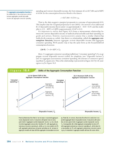
ing when Y D equals zero. This is the relationship represented in Figure 16.4 by CF, anal-
ogous to cf in Figure 16.3.

figure 16.4 Shifts of the Aggregate Consumption Function

(a) An Upward Shift of the (b) A Downward Shift of the
Aggregate Consumption Function Aggregate Consumption Function
Consumer Consumer
spending, C spending, C
Aggregate Aggregate
consumption consumption
function, CF 2 function, CF 1

Aggregate Aggregate
consumption consumption
function, CF 1 function, CF 2

A 2 A 1

A 1 A 2

Disposable income, Y D Disposable income, Y D

Panel (a) illustrates the effect of an increase in expected aggregate up. Panel (b), in contrast, illustrates the effect of a reduction in ex-
future disposable income. Consumers will spend more at every pected aggregate future disposable income. Consumers will spend
given level of aggregate current disposable income, Y D . As a result, less at every given level of aggregate current disposable income,
the initial aggregate consumption function CF 1 , with aggregate au- Y D . Consequently, the initial aggregate consumption function CF 1 ,
with aggregate autonomous consumer spending A 1 , shifts down to
tonomous consumer spending A 1 , shifts up to a new position at CF 2
with aggregate autonomous consumer spending A 2 . An increase in a new position at CF 2 with aggregate autonomous consumer spend-
aggregate wealth will also shift the aggregate consumption function ing A 2 . A reduction in aggregate wealth will have the same effect.

164 section 4 National Income and Price Determination