Page 223 - Krugmans Economics for AP Text Book_Neat

fact, industry analysts often talk about variations in an industry’s “pricing power”:
The short -run aggregate supply
when demand is strong, firms with pricing power are able to raise prices—and they do.
curve shows the relationship between
Conversely, if there is a fall in demand, firms will normally try to limit the fall in the aggregate price level and the quantity
their sales by cutting prices. of aggregate output supplied that exists in
Both the responses of firms in perfectly competitive industries and those of firms in the short run, the time period when many
imperfectly competitive industries lead to an upward -sloping relationship between ag- production costs can be taken as fixed.
gregate output and the aggregate price level. The positive relationship between the ag-
gregate price level and the quantity of aggregate output producers are willing to supply
during the time period when many production costs, particularly nominal wages, can
be taken as fixed is illustrated by the short -run aggregate supply curve. The positive Section 4 National Income and Price Determination
relationship between the aggregate price level and aggregate output in the short run
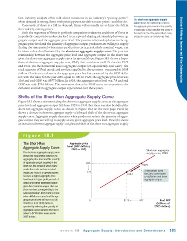
gives the short -run aggregate supply curve its upward slope. Figure 18.1 shows a hypo-
thetical short -run aggregate supply curve, SRAS, that matches actual U.S. data for 1929
and 1933. On the horizontal axis is aggregate output (or, equivalently, real GDP)—the
total quantity of final goods and services supplied in the economy—measured in 2005
dollars. On the vertical axis is the aggregate price level as measured by the GDP defla-
tor, with the value for the year 2005 equal to 100. In 1929, the aggregate price level was
10.6 and real GDP was $977 billion. In 1933, the aggregate price level was 7.9 and real
GDP was only $716 billion. The movement down the SRAS curve corresponds to the
deflation and fall in aggregate output experienced over those years.

Shifts of the Short -Run Aggregate Supply Curve

Figure 18.1 shows a movement along the short -run aggregate supply curve, as the aggregate
price level and aggregate output fell from 1929 to 1933. But there can also be shifts of the
short -run aggregate supply curve, as shown in Figure 18.2 on the next page. Panel (a)
shows a decrease in short -run aggregate supply—a leftward shift of the short -run aggregate
supply curve. Aggregate supply decreases when producers reduce the quantity of aggre-
gate output they are willing to supply at any given aggregate price level. Panel (b) shows
an increase in short -run aggregate supply—a rightward shift of the short -run aggregate supply

figure 18.1

The Short -Run Aggregate price
Aggregate Supply Curve level (GDP deflator,
2005 = 100) Short-run aggregate
The short -run aggregate supply curve supply curve, SRAS
shows the relationship between the
aggregate price level and the quantity
of aggregate output supplied in the 10.6
short run, the period in which many 1929
production costs such as nominal A movement down
wages are fixed. It is upward sloping 7.9
1933 the SRAS curve leads
because a higher aggregate price to deflation and lower
level leads to higher profit per unit of aggregate output.
output and higher aggregate output
given fixed nominal wages. Here we
show numbers corresponding to the
Great Depression, from 1929 to 1933:
when deflation occurred and the ag-
gregate price level fell from 10.6 (in 0 $716 977 Real GDP
1929) to 7.9 (in 1933), firms re- (billions of
sponded by reducing the quantity of 2005 dollars)
aggregate output supplied from $977
billion to $716 billion measured in
2005 dollars.

module 18 Aggregate Supply: Introduction and Determinants 181